
Bengt J. Olsson
LinkedIn: beos
X/Twitter: @bengtxyz
A short discussion on the principles for determining electricity prices and flows within the European power system. Basically, for each quarter of an hour an optimization problem, spanning the supply and demand in most of Europe, is solved by an algorithm named EUPHEMIA.
This LinkedIn article provides a high level introduction to the subject. The text of the article is also provided below.
TL;DR
Discussions about electricity prices, congestion income, and cross-border trade are often framed in political or distributional terms — who gains, who loses, and whether outcomes are “fair”. What is sometimes missing is a clear understanding of what the market is actually optimizing.
European electricity prices are derived by maximizing welfare: consumer utility minus production cost, subject to market balance and network constraints. In a flow-based framework, internal and cross-border grid constraints are represented via PTDF matrices acting on zonal net positions. Prices, flows, and congestion income are results of this constrained welfare maximization — not objectives in themselves.
This welfare maximization is as close as one can get to a market outcome driven purely by supply and demand, given the physical constraints of the power system. Any attempt to alter the outcome therefore inevitably introduces some form of price or quantity regulation.
Why zonal pricing is harder than it looks
Deriving zonal electricity prices and flows is not an easy task, nor is it particularly intuitive. Before flow-based capacity calculation, power flows followed the price gradient, moving from lower-price zones to higher-price zones. With the introduction of flow-based market coupling, flows are determined not only by economic incentives but also by the physical characteristics of the power system, as captured by power transfer distribution factors (PTDFs). This dual steering, economic and physical, makes power flows significantly less intuitive to interpret.
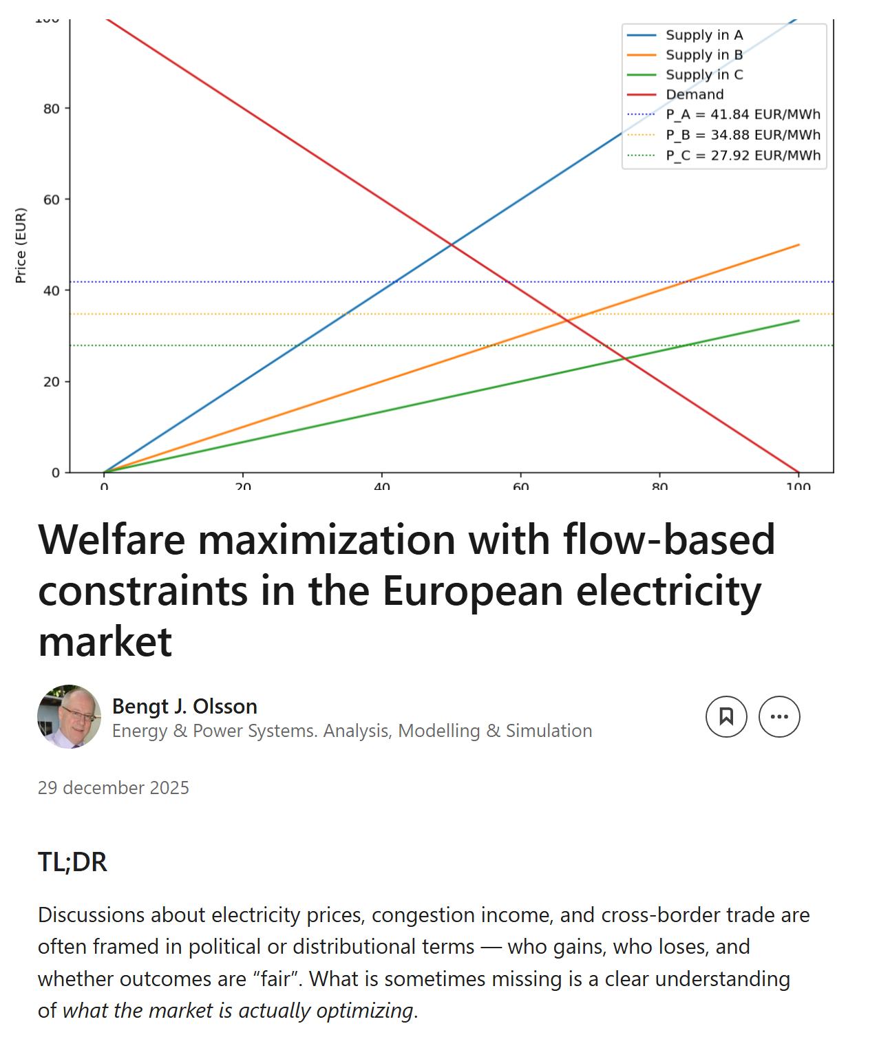
To better understand the mechanics myself, I have broken the problem down and applied it to a simple, computable model consisting of:
- A small network (three zones with three interconnections)
- A single internal constraint within one zone
- Linear demand and supply curves
- Simple impedances on each link (and on the constraint), allowing the construction of a PTDF matrix
But first a short look at the theoretical framework, in a simplified and principal manner, not taking into account all the variations, such as different bid forms etc. that the real algorithms must handle.
The optimization problem behind European electricity prices
In Europe, electricity prices are derived from an algorithm called EUPHEMIA, which solves an optimization problem. In simplified form, the objective can be written as:
W = max(U − C)
where welfare (W) is maximized as the difference between utility (U) and cost (C).
Utility represents the aggregated willingness of consumers to pay for electricity. Cost represents the aggregated cost (as bid) for producers to supply electricity.
In welfare terms, U − C represents the economic value added created by the market.
What “utility” and “cost” actually mean
“Aggregated” here means integrated over volume.
Utility (U) is the area under the marginal demand curve up to the cleared demand volume d. Cost (C) is the area under the marginal supply (marginal cost) curve up to the cleared supply volume s.
Total U is the sum of all zonal utilities, and total C is the sum of all zonal costs. The cleared supply and demand in each zone are the variables chosen by the optimization.
Net position: the key coupling variable
For each zone, the difference between supply and demand is called its net position (NP):
NP = supply − demand
Net position is a central concept in market coupling:
- NP > 0 means the zone is a net exporter
- NP < 0 means the zone is a net importer
Across all zones, the market must balance:
Sum of all NP = 0
This expresses the fact that total production equals total consumption and acts as a constraint in the optimization.
Market balance provides the first constraint to the maximization problem.
Where flow-based constraints enter
The second major class of constraints concerns the power grid itself.
In flow-based market coupling, network constraints that limits the power transmission capacity, can be located anywhere in the system, not only at zone borders. The optimization must therefore respect both cross-border and internal grid constraints.
Using the flow-based method, flows on constrained network elements are represented by:
Flow on constrained elements = PTDF matrix × NP vector
How the PTDF matrix works
The PTDF matrix has constrained network elements as rows and zones as columns.
Each PTDF value represents how a one-megawatt increase in net position in a given zone — balanced by a corresponding decrease in a reference (slack) zone — affects the flow on a specific constrained network element.
The matrix multiplication gives the combined effect of all zonal net positions on all constrained resources. These effects must remain within the physical capacity limits of the network.
Network constraints provides the second class of constraints to the maximization problem.
From optimization to prices and physical flows
Solving the optimization problem determines:
- Cleared supply and demand in each zone
- Zonal prices
- Zonal net positions
Using the net positions together with the PTDF matrix, the corresponding flows on constrained network elements can be calculated.
In practice, one may also introduce non-binding “monitoring” elements on zonal borders, with sufficiently high capacity so that they never bind, but with well-defined PTDF coefficients. This allows the calculation and reporting of implied inter-zonal border flows from the zonal net positions, even though these elements do not influence the market clearing.
Welfare decomposition: CS, PS, and CI
A common way to present the result is to decompose welfare as:
W = CS + PS + CI
where:
- Consumer surplus (CS) is consumer utility minus payments
- Producer surplus (PS) is revenues minus production costs
- Congestion income (CI) reflects the value of scarce network capacity
Note that the maximization of welfare, max(U-C), does not need the concept of a zonal price, and in EUPHEMIA, the “master problem” does not provide zonal prices. In principle it is trivial to get the zonal prices when zonal demand and supply is established, but they are not needed in the first welfare maximization step. But in order to decompose W into CS, PS and CI the zonal prices must be established, which gives an indication that CS, PS and CI are derived entities from max W.
Formally, congestion income is linked to the shadow prices of binding network constraints, as the sum (over all binding constraints) of shadow price x RAM (Remaining Available Margin). This total CI can be decomposed as as the sum of border flows multiplied by the price differences between connected zones. This decomposition provides a certain familiarity to the older ATC/NTC method of calculating CI, but should be used with caution and with an understanding of the real reasons for CI, otherwise wrong conclusions may be drawn.
A common misunderstanding about congestion income
Because welfare can be written as W = CS + PS + CI, it is sometimes assumed that congestion income itself is part of the optimization objective — that welfare increases by maximizing price differences or cross-zonal flows.
This is incorrect.
Congestion income is caused by maximizing utility minus cost subject to network constraints. It is not an objective in itself, but a consequence of constrained network resources.
If one dislikes congestion income, what one really dislikes is the existence of binding grid constraints — because those constraints are what generate congestion income in the first place.
Next: the model and the results
If you want to see this framework applied in practice, please have a look at the model and results presented here: https://adelsfors.se/2025/04/08/the-three-zone-market-using-flow-based-constraints/
That blog also links to similar two- and three-zone models using the conceptually simpler NTC/ATC approach, where constraints are placed only on zone borders.
For a more intuitive explanation of PTDF matrices, see this analogy between power flows in AC networks and current flows in resistive DC circuits: https://adelsfors.se/2025/04/04/power-flow-meets-ohms-law-a-simple-ptdf-analogy/