Power Flow meets Ohm’s Law: A Simple PTDF Analogy

Bengt J. Olsson
Twitter: @bengtxyz 
LinkedIn: beos

The DC power flow model is used to calculate Power Transfer Distribution Factors (PTDF) in power networks. The model approximates the real AC power flows by linearizing the governing equations, that are expressed in voltage angles and impedances. Also the resistive part of the impedances is assumed to be zero, to not have to deal with power losses. Despite this, it provides a good first-order approximation of the active AC power flow.

Now the DC power flow is mathematically equivalent to the current flow in a resistive electrical circuit. This analogy is very useful for understanding the basic principles of power flow by relating them to a simpler, more intuitive concept such as current in a resistive network.

In this analogy voltage angles, susceptibilities and power flows in the DC power flow model are substituted with voltages, conductances and currents in a resistive electric circuit. The analogy offers an intuitive way to understand Power Transfer Distribution Factors (PTDFs).

The results here can probably be described as a simplified and implicit subset of the findings in this paper.

Analogy Table:

DC power flow (AC)	Resistive DC Circuit	Interpretation
Pij = Bij * (θi−θj)	Iij = Gij * (Vi−Vj)	Flow driven by potential difference.
Susceptance B=1/X	Conductance G=1/R	Reciprocal of reactance/resistance
Phase angle difference θ	Voltage difference V	Generalized potential
Active power flow Pij	Current flow Iij	What is actually flowing
Slack bus/node	Ground node	Phase angle is zero in the slack bus/node, as is the voltage in the ground node.
Power flow is conserved	Charge (current flow) is conserved	Conserved flows, no losses
Linearized model	Ohm’s Law	Both result in linear relationships
PTDF	Normalized branch currents	Normalized branch currents gives the corresponding PTDFs

How to use this analogy to compute PTDFs:

1. Build a resistive circuit:
   Connect nodes using resistors, one per transmission line. Use R = X (reactance becomes resistance).
2. Select a slack node:
   Set one node (e.g., node 1) to 0V. It will absorb all current (i.e., power). The slack bus corresponds to the ground node in an electrical circuit.
3. Inject 1V at another node:
   For example, set node 2 to 1V and keep others unknown (except slack = 0V).
4. Solve for node voltages:
   Apply Kirchhoff’s Laws (KCL/KVL) to find voltages at all other nodes.
5. Calculate currents:
   Use I_ij = (V_i – V_j) * G_ij = (V_i – V_j) /R_ij for each branch. Keep track on current flow directions in relation to the flow definitions!
6. Normalize:
   Compute total outgoing current from the injection node. Divide all branch currents by this total to get the corresponding PTDFs.

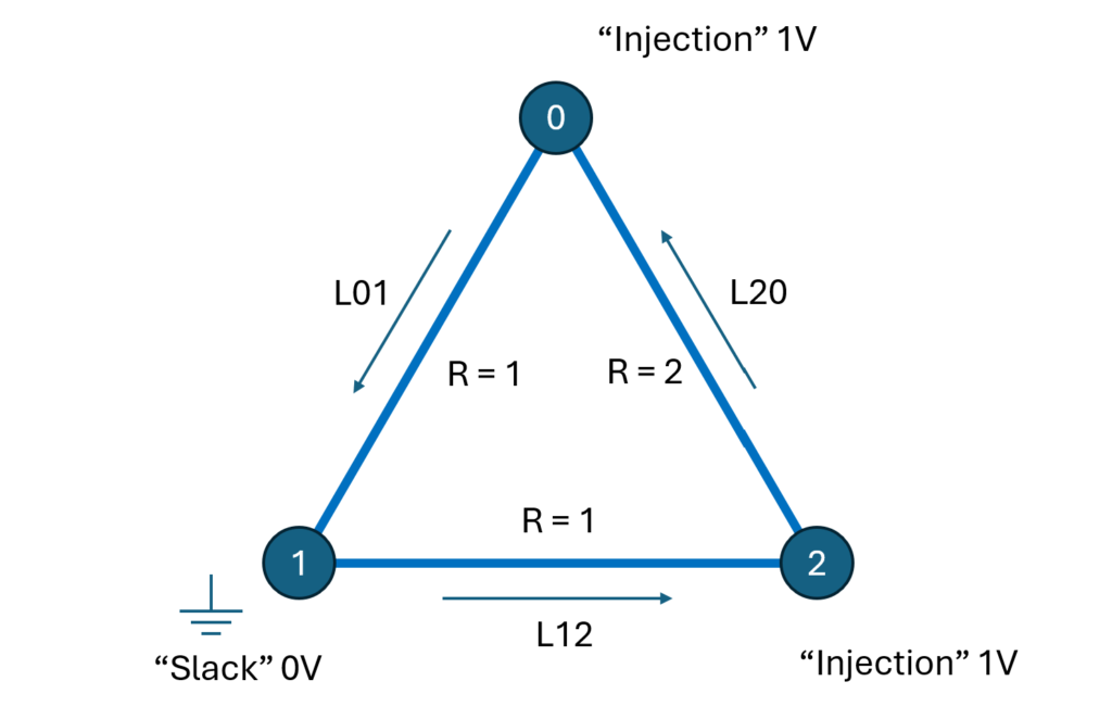
Example

For the triangle network above we can do like this:

• Inject 1V in node 0.
• The electric network then looks like 1V in node 0 is connected to ground (slack bus/node 1) via two paths
  • one with 1 ohm resistance and
  • a second with 1 + 2 = 3 ohms.
• Through the first path we have 1 A and through the second 1/3 A. Together we have 4/3 A emitted from node 0.
• Normalize the outgoing currents by dividing them with 4/3.
  • Then 3/4 A flows from node 0 to node 1,
  • and 1/4 A flows from node 0 via node 2 to node1.
• Considering the defined directions in the figure the first column (injection in bus/node 0) of the PTDF matrix then becomes [ 3/4 -1/4 -1/4 ] (transposed). By doing the same calculations for injection in node 2, the following PTDF matrix is obtained.

PTDF matrix	Injection in Node 0	Node 1 (slack)	Injection in Node 2
Link 0 -> 1	3/4	0	1/4
Link 1 -> 2	-1/4	0	-3/4
Link 2 -> 0	-1/4	0	1/4

Result:

• Each normalized current represents the PTDF for that branch.
• The PTDF matrix has:
  • Rows = links
  • Columns = buses/nodes
  • Values = flow per MW injected