
Bengt J. Olsson
Twitter: @bengtxyz
LinkedIn: beos
Introduction
Model
Scenarios
Results
Discussion
Conclusions
Introduction
Sweden’s future power system must accommodate up to 300 TWh of electricity consumption per year in the future according to many analysts. This is also often mentioned in the press. This is more than double the consumption of today which is about 140 TWh. Typical production today is around 170 TWh which means that 30 TWh is (net) exported. Out of the projected 300 TWh consumption about 100 TWh are allocated for green hydrogen production to mainly the steel industry but to others as well. This leaves 200 TWh or for “ordinary” consumption, an increase with 60 TWh from today. It is not evident how to use up all these extra TWhs. With about 8 Gmil (a Swedish “mil” equals 10 km) accumulated road distance and 2 kWh per mil, about 16 TWh more electrical power is consumed when all cars are electrified. Electrified heating with heat pumps instead of biomass combustion will consume another chunk.
Anyway, these are the numbers that will be used. Note that the 100 TWh consumed for green hydrogen will provide about 70 TWh of the hydrogen measured in its calorimetric value, (Lower Heating Value, LHV) which is often used when discussing quantities of hydrogen.
But here the energy amount used to produce the hydrogen is used as the measure of hydrogen quantity, since we are mainly interested in the power system impact of this production.
The model
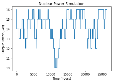
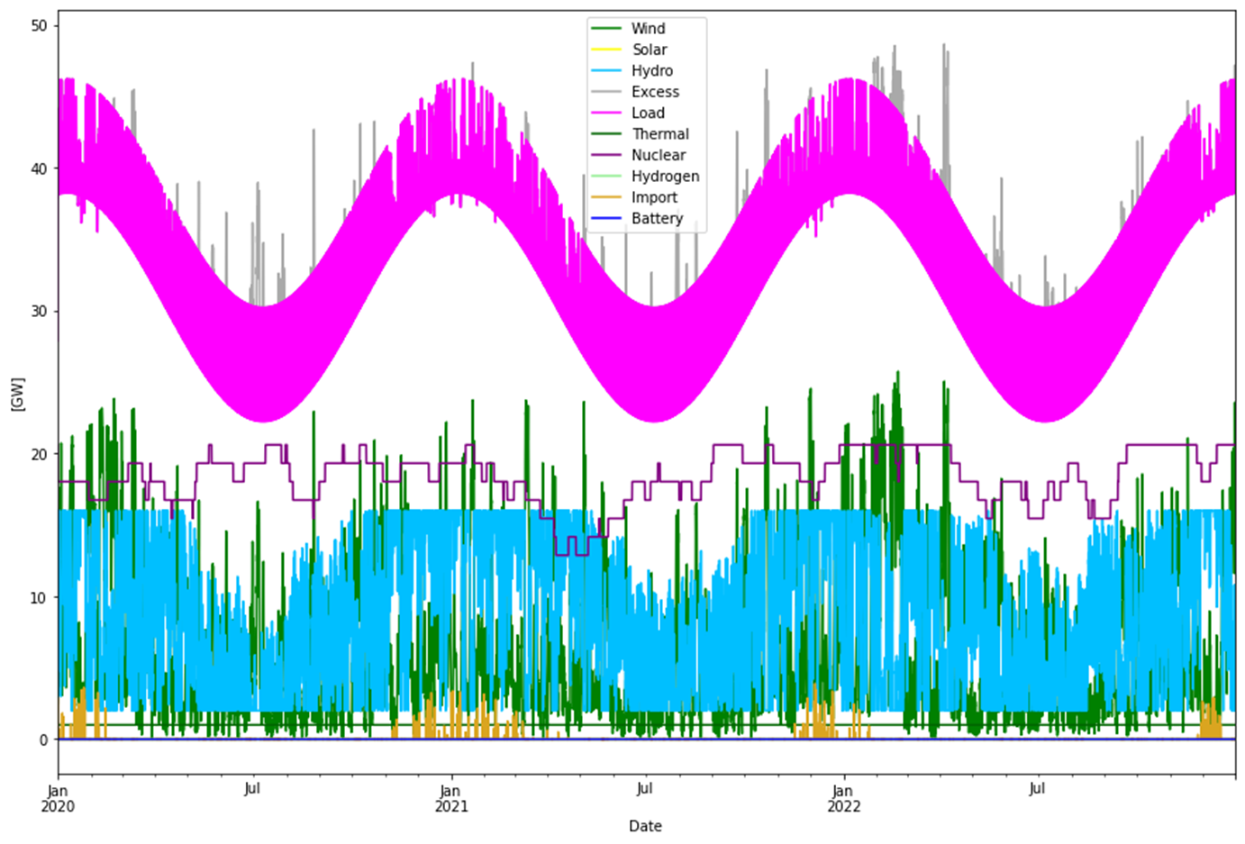
The model is a balance model that hour-by-hour balances supplied power with consumed power. Real power production data is used for onshore/offshore wind and solar/PV power. The data is taken from ENTSO-E for Germany 2020-2022. It doesn’t really matter so much from which country the data is taken, the intention is to get “typical” patterns of onshore wind, offshore wind and solar/PV power production. (You could potentially have a weather pattern in Sweden that matches the used German pattern). These are then first assigned reasonable capacity factors (here 50% for offshore wind power, 30% for onshore and 11% for solar/PV power) and then scaled up and down to minimize the cost of the total system. And Germany has the most statistics of our neighboring countries. Simulated power dispatch is used for nuclear power, see picture below. Swedish hydro power (augmented with Norwegian import) is modeled as flexible power source with a delivery range 2-16 GW. Thermal power (mostly biomass) is considered a fixed power source at 1 GW (number taken from Swedish TSO model for 2050; 9 TWh per year, indicating a change-over from biomass to heat-pumps for district heating and similar). Hydrogen CCGT is modeled as a flexible power source fueled by stored hydrogen.
Consumption is modeled into two parts. First there is the “normal” consumption. It is modeled as sinusoidal over the year with max in the winter and min in the summer. Overlaid is a sinusoidal over a day, with maximum at 15:00 and min at 03:00. The sum of this consumption over the year is 200 TWh. Not a super-realistic demand model but good enough since the effects we’re looking at stretches over longer times and then the daily variations are not that important. But from a peak power perspective, it will underestimate the peaks having the smooth sinusoidal shape. Electric Vehicles (EV) and heat stores will move consumption from day to night and hence give the daily sinusoidal less amplitude.
The other part (about 100 TWh) is consumption due to production of hydrogen for industrial purposes. This production is considered as 100% flexible, except when the hydrogen store reaches an empty level. Then a production level will be maintained at 50% of the nominal production. The nominal production is 100/8.76 = 11.4 GW. Hence the minimum production level will be 5.7 GW which then always will be deliverable for the industry. The drawback with this is that 5.7 GW of flexibility is lost when it is needed most (empty storage implies negative power balance). On the other hand, the cost for society is considered higher if hydrogen production is shut down completely.
Storages are modelled as objects with attributes power in and out capacities, a size and a round-trip efficiency. An update fill level method provides the current fill level of each storage.
For each simulation of the three years 2020-2022, a set of scale factors are decided that scales the power sources and other resources. The automatic optimization procedure (below called the “solver”) finds the set of scale factors that provides the minimum cost for the total system, given two boundary conditions:
- No deficit shall occur (excess is OK, this will be curtailed or exported, but deficits must not occur)
- Power sources are scaled such that max 74 TWh of the flexible hydro power is produced, corresponding to a normal year of 67 TWh (Sweden) + 7 TWh (import from Norway).
The hydrogen store is used both for storing hydrogen for delivery and for balancing the power system, in a sort of sector coupled system. The requirement is to be able to deliver 100 TWh per year at a steady rate to the industry but also to provide a flexibility service for the power system. Hydrogen production and storage quantities are measuered in terms of input energy, i.e. the energy needed to produce the quantity. The conversion between input energy and H2 LHV energy as a measure for energy stored is given by these chosen values for hydrogen production:
- 50 kWh -> 1 kg H2 (in electrolyzer production)
- 1 kg H2 <-> 33.3 kWh (LHV)
- 1 kg H2 -> 20 kWh (in CCGT generation)
Hence 100 TWh consumed electric energy provides 67 TWh of LHV H2 (33.3/50 or 2/3 * 100). It can also be seen that the round-trip efficiency of power->hydrogen->power becomes 20/50 or 40%.
Battery stores have been considered but the solver usually excludes these in the optimization, probably due to their high cost of storage capacity when compared to hydrogen storage. In the final optimization these are excluded due to their low impact on the system, and hence make the parameter space simpler to optimize by the solver. In a more refined model that for instance considers rate limits on CCGTs or hydropower they would probably have more impact.
Hydropower is modelled as a flexible source with a capacity between 2 and 16 GW. (3 GW and 7 TWh are imported from Norway, that almost become part of the Swedish hydropower system). See this blog for details.
Typically import and export are not part of the model since they (especially import) introduce a high level of “arbitrarytness” given the complex interaction with the outside world. Anyway here, as a last resort, 7 GW of import is included and always expected to be available. (Sweden has 10 GW import capacity but 3 GW are used by the Norweigan hydro import as mentioned above). A high cost per kWh, “scarsity pricing”, is assigned to this import (since needed when RE resources are low which tends to give a high price) so the solver may not use all import capacity, but instead build out power production (which is really what is wanted for power security reasons).
Transmisson costs are not part of the model, it is assumed that there are no transmission limitations. Neither are other system costs that are needed to maintain a safe operation of the system.
Cost model
CAPEX and OPEX costs are the same as in the previous blog using the same model. For nuclear power, the “Nuclear 5” values are used, that is a CAPEX cost of 5 GUSD/GW and a yearly OPEX cost of 200 MUSD/GW. Offshore wind power is adjusted down from 3 to 2.5 GUSD/GW. It is assumed that Sweden has 16.3 GW of installed onshore and zero offshore wind power, 2 TWh Solar/PV power and 7 GW nuclear power today (and of course no hydrogen storage, electrolyzers or hydrogen CCGT). These capacities are subtracted from the resulting capacities to provide the actual remaining cost to reach the scenarios. Hydro power and Thermal (Biomass/heat/waste etc) are considered as “sunk cost” and are not included in the cost calculations. Values in USD, translated to SEK @ 10 SEK / USD.
The evaluated scenarios
Four cases or scenarios will be analyzed
- Present level of nuclear power with increased level of renewable energy (RE) and with hydrogen bulk storage
- Optimized levels of nuclear power and RE and with hydrogen bulk storage
- Present level of nuclear power with increased level of RE and with hydrogen buffer storage
- Optimized level of nuclear power and RE and with hydrogen buffer storage
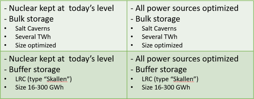
The reason for choosing this evaluation matrix is to understand the differences when either adding only more renewable or adding both more renewable and nuclear power. Also to examine on one hand the impact of hydrogen storage in bulk (meaning a storage that can do seasonal storage and is in principle never empty), like large salt caverns. And on the other hand, a hydrogen buffer store that handles short time variations (and hence relies on a less variable production and/or consumption). Bulk storage typically has several TWh in storage capacity. The size of the bulk storage is an optimization parameter. The buffer storage is limited to a size between 16-300 GWh. 16 GWh is of the order of what the Skallen LRC (Lined Rock Cavern) in southern Sweden (the only of its kind in the world). 300 GWh corresponds roughly to two of the large LRCs that have been discussed in the media in relation to the HYBRIT project for direct reduction of iron ore.
Results
Generation results for the four cases are summarized in the graph below. For each case, the power generation (source) and consumption (sink) balance are shown.
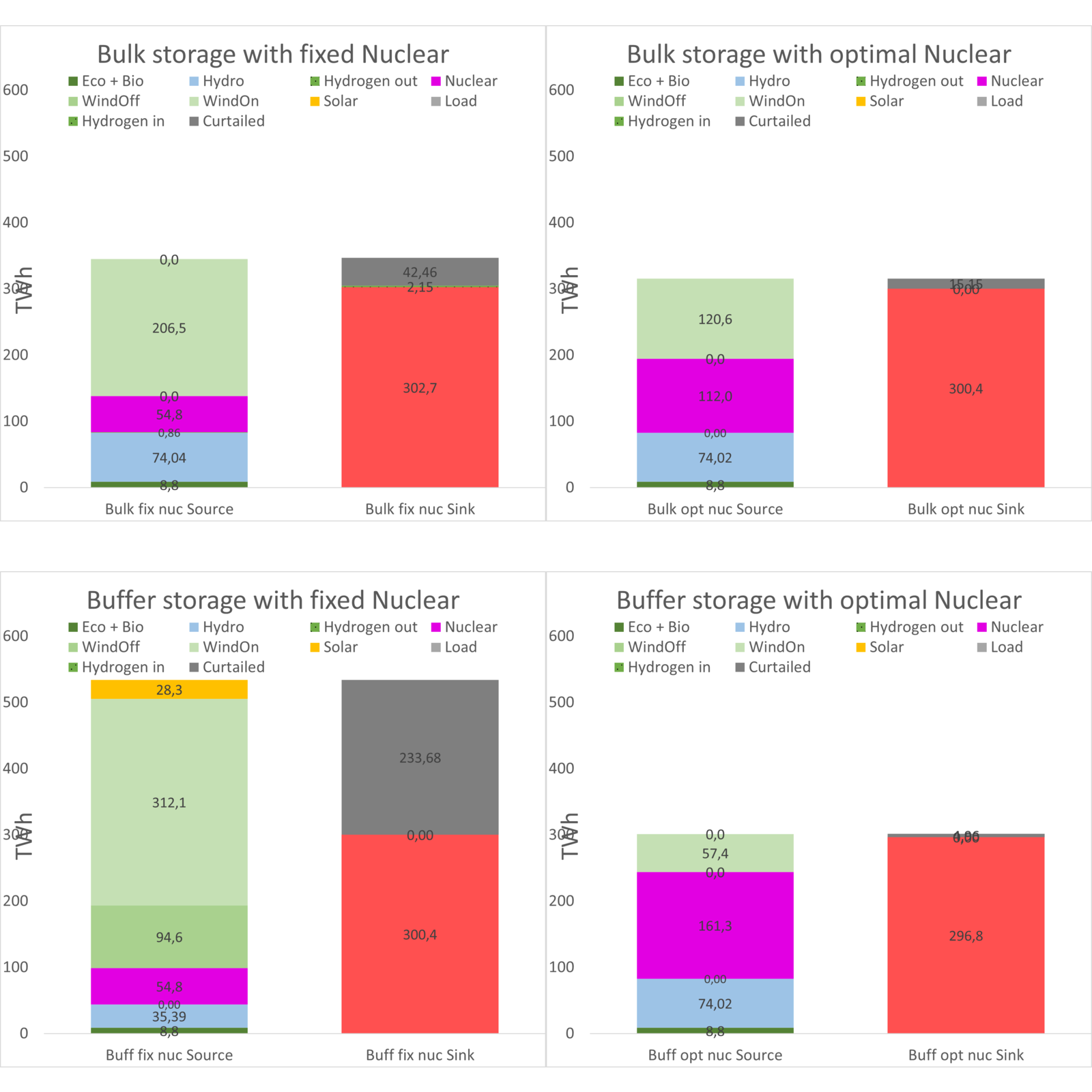
| Fixed Nuclear ( = 7 GW / 55 TWh) | Optimal Nuclear | |
| Bulk Storage | Storage size: 4.7 TWh Renewable energy: 207 TWh Nuclear energy: 54.8 TWh Curtailed energy: 42.5 TWh Electrolyzer capacity: 23.4 GW (50% utilization) Hydrogen CCGT capacity: 4.7 GW (2.1% utilization) Build-out CAPEX cost: 83.9 GUSD System LCOE: 63.6 USD/MWh (öre/kWh) | Storage size: 4.8 TWh Renewable energy: 121 TWh Nuclear energy: 112 TWh (7.3 GW build-out) Curtailed energy: 15.2 TWh Electrolyzer capacity: 16.1 GW (71% utilization) Hydrogen CCGT capacity: 0 GW Build-out CAPEX cost: 83.7 GUSD System LCOE: 62.5 USD/MWh (öre/kWh) |
| Buffer Storage | Storage size: 300 GWh Renewable energy: 435 TWh Nuclear energy: 54.8 TWh Curtailed energy: 233.7 TWh Electrolyzer capacity: 19.6 GW (58% utilization) Hydrogen CCGT capacity: 0 GW Build-out CAPEX cost: 180.5 GUSD System LCOE: 108.7 USD/MWh (öre/kWh) | Storage size: 16 GWh Renewable energy: 57 TWh Nuclear energy: 161 TWh (13.6 GW build-out) Curtailed energy: 5.0 TWh Electrolyzer capacity: 11.4 GW (96% utilization) Hydrogen CCGT capacity: 0 GW Build-out CAPEX cost: 79.3 GUSD System LCOE: 63.0 USD/MWh (öre/kWh) |
Discussion
Bulk storage cases
The two bulk storage cases come in at about the same build-out cost and System LCOE. That is, given the availability to about 5 TWh of hydrogen bulk storage (in salt caverns) both scenarios give the same outcome. The fully optimized (more nuclear) does not utilize any hydrogen CCGT for power balancing, it is enough to use the available hydropower for balancing. In the RE rich alternative a certain amount of CCGT is needed to complement the hydropower for balancing out the higher variability. The curtailed energy is also higher in the RE rich scenario. Nuclear build-out in the optimal scenario is 7.3 GW (that is a to a total of 14.3 GW).
A big problem with the bulk storage alternatives is that since the storage needs are weather dependent, the storage must really be designed for the worst-case production deficit due to an extended period of low wind which is shown by Ruhnau/Qvist. This means that real bulk storage will be much larger (probably 2-3 times larger) to cope with the worst-case weather period. But you can never know…
The other main problem with these alternatives is that Sweden does not have the geological conditions for building salt cavern bulk hydrogen storages at all…
Buffer storage cases
Here the difference between “fixed nuclear” (that is “RE rich”) and “optimal” is huge! In fact, the RE rich scenario becomes completely unreasonable. Since there is no bulk storage of hydrogen, this scenario becomes susceptible to seasonal variations in RE production and load. During the high load seasons the production capacity is too low. Since the buffer storage is quickly emptied there is no backup possibility from burning hydrogen, no matter how much CCGT capacity is available. There is no fuel for these CCGTs. The solver hence throws in a lot of expensive offshore wind power capacity to “lift” the floor of power production during the winter seasons.
This could of course be compensated by adding other plannable production resources, such as biomass fueled turbines or increasing the maximum power from the hydropower part. This has not been part of this study, but this would add a substantial cost as well. (A simple run with increasing the hydropower max power to 26 GW instead of 16 GW gave a build-out cost of 116 GUSD or 33-37 GUSD higher than in the other cases, plus the cost for adding 10 GW hydro power. This is not an option).
The optimal scenario with more nuclear instead gave a cost in line with the bulk hydrogen build-out and production costs. The cost is here shifted from the bulk storage/electrolyzers/CCGT costs to build more nuclear power instead. Nuclear power build-out in this scenario is from 7 GW today to 20.6 GW, that is an increase with 13.6 GW.
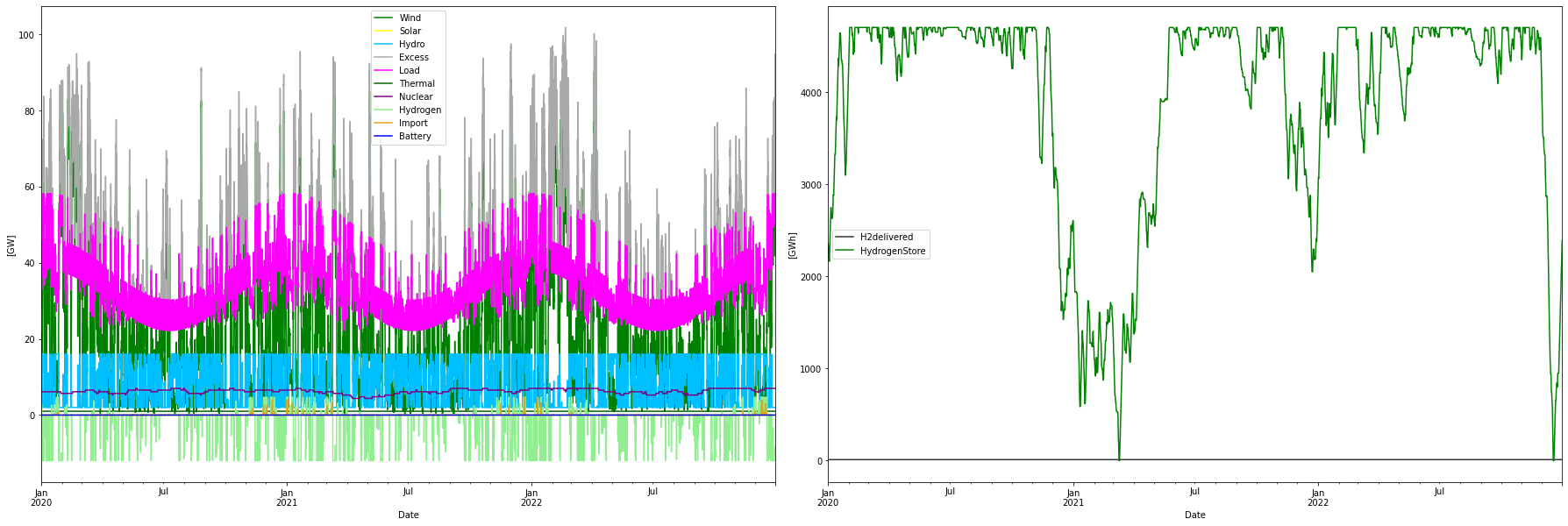
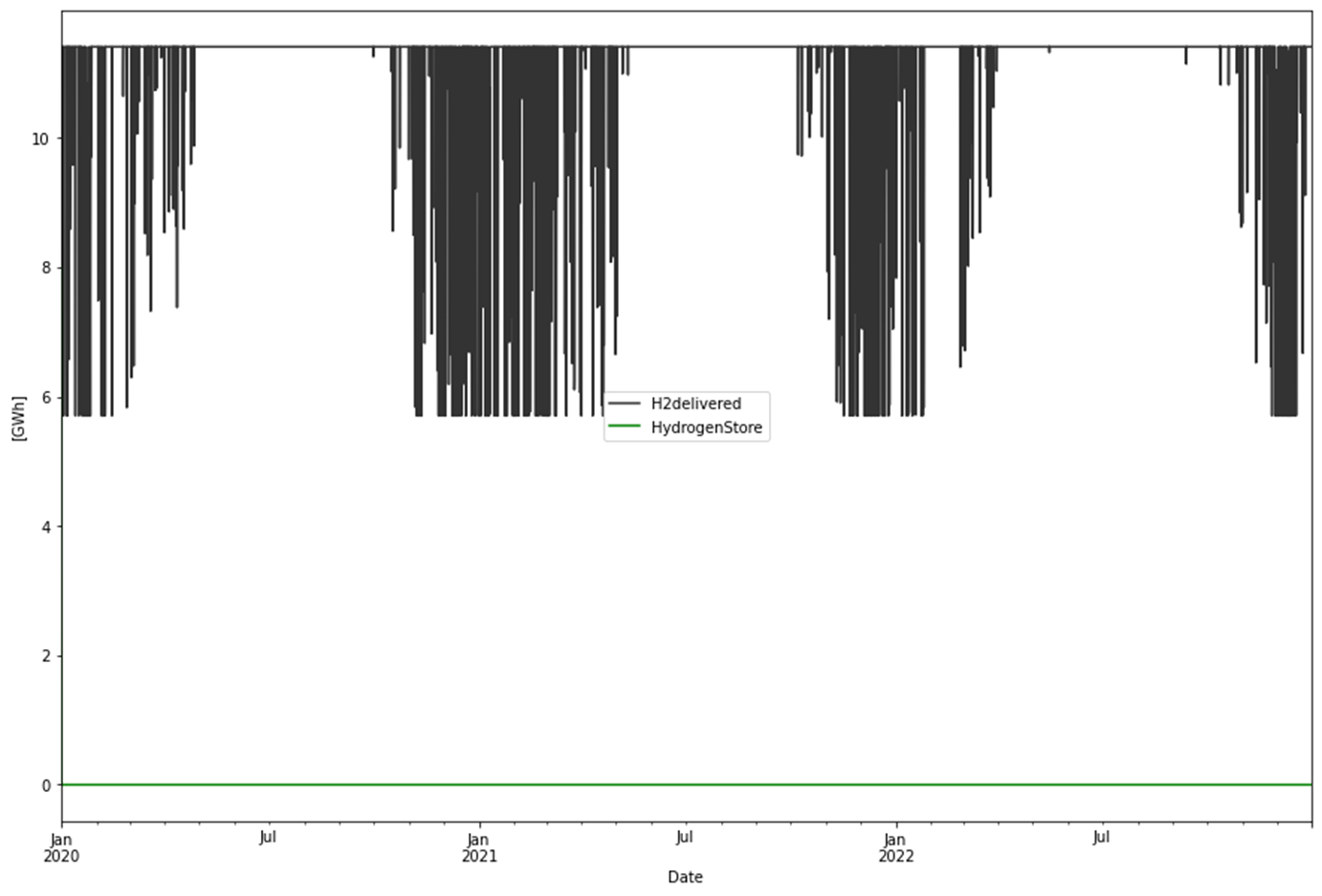
Another difference is that the solver dictated the largest buffer store (300 GWh) for the RE rich alternative (which is to be expected since it relies on that store also for power balancing). But for the optimal, nuclear rich, scenario the solver suggested the smallest buffer store, 16 GWh. In this case, 11.4 GW of electrolyzer capacity is run at 96.4% utilization (that is full utilization all the time except the 3.6% of the time when it needs to flex down to save power). In theory no store at all would be needed in this case since all hydrogen is delivered immediately after it is produced. In the simulation, at least a 11.4 GWh store is needed since production and delivery is done in sequence, and the process is sampled one time per hour.
Hydrogen delivery will never be perfect when the buffer size is limited, and flexible production is used. Production will flex down from time to time to save power and hydrogen may not be available in the buffer. In the 16 GWh buffer storage case the delivery will be above 10 GW for 90% of the time but will occasionally flex down more as seen in the picture below. In total 3.6 TWh of the 100 TWh production are lost with this flexibility.
If hydrogen should be produced in excess to be used during the deficit hours, the store must be much larger and in fact become a bulk storage.
Conclusions
Out of the four investigated hydrogen storage and power build-out combinations only one is real-world compatible given the conditions presented above. It is the small hydrogen buffer storage alternative, matched with a large nuclear power build-out and a smaller onshore wind power build-out. In this scenario almost 13.6 GW of nuclear power and 5.5 GW of onshore wind power is added to the present power system to serve 200 TWh of “normal” consumption plus 100 TWh (70 TWh H2 LLV) hydrogen production for the industry. A 16 GWh hydrogen buffer store is used (size of the “Skallen” natural gas LRC store in southern Sweden) to deliver the produced hydrogen at a steady state rate at 11.4 GW but around 3% of the time the rate will flex down to 5.7 GW.
The two bulk store alternatives go away since Sweden cannot house 5 TWh hydrogen salt caverns (or possibly double this amount considering a worst-case weather scenario, not done here). Building this kind of bulk store with LRCs is not an option.
The buffer store (300 GWh) alternative with only build-out of renewable energy also goes away since it cannot handle power/energy deficits in the winter seasons, unless built out with unreasonable amount of onshore, offshore and solar/PV power. The indicated cost given the assumptions above is more than double that of any of the other alternatives.
Offshore wind production was excluded by the solver in all cases except in the “pathological” case of the fixed 300 GWh buffer store and large RE build-out. Typically, the solver reasons that the difference in wind power pattern between onshore and offshore wind is too small to motivate a build-out with offshore wind power when it can build onshore windpower for a much lower cost. The CAPEX costs are here set to 1 and 2.5 GUSD/GW for onshore and offshore wind power respectively, and if that ratio changes then offshore wind could play a part.
Likewise, the contribution of solar/PV was also excluded from the three theoretically viable cases. In the 16 GWh buffer/nuclear build-out case this is quite understandable since solar does not contribute during the winter and there is no seasonal storage. It is a little bit harder to understand why it does not contribute in the bulk storage scenarios. But it is probably simply because the levelized cost of production is higher for solar at 0.5 GUSD/GW with 11% capacity factor than for onshore wind at 1 GUSD/GW and 30% capacity factor. Since the bulk store can store any of these power types it stores what is cheapest to produce. A similar conclusion was reached by Qvist et al in their work “Kraftsamling 2050”.