
Bengt J. Olsson
Twitter: @bengtxyz
LinkedIn: beos
In the last blog post, I compared the Solar/Wind/Eco/Nuclear/Storage (“SWENS”) model with a similar model described by Ruhnau/Qvist (“RQ”), using as similar cost parameters and other presumptions as possible. While the RQ model is much larger in scope than my simpler SWENS model (remember, this is a blog, not a scientific paper… 😉 ) the outcome was very similar. This comparison provided a benchmark that encourages further exploitation of the SWENS model.
In this blog post I have the following objectives:
- Using updated (more realistic?) costs in the SWENS model
- Using enhanced (higher) capacity factors for wind and solar power
- Including nuclear power in the power system mix at different cost levels
As in the RQ paper, a Germany with 540 TWh of consumption is modelled, but the time series used here is real wind and solar power production data for 2020-2022. Four cases will be investigated, all with the same cost parameters, except for cost of nuclear power, that will differ in each case:
- No Nuclear: No nuclear power at all included in the power mix
- Nuclear 4: Nuclear power included at a cost of 4 GUSD/GW
- Nuclear 5: Nuclear power included at a cost of 5 GUSD/GW
- Nuclear 5.5: Nuclear power included at a cost of 5.5 GUSD/GW
Please take the results for what they are: The outcome of a coarse model with many real-world properties not factored in. But hopefully it will contribute to the general perspective by showing and comparing how different power sources contribute to the total system. Also, of course the outcome is completely dependent on the used cost levels and capacity factors as described below.
Results
The energy bar chart shows the optimal produced (source) and consumed (sink) energies from the different power sources and sinks. That is, optimal in the sense that the shown power mixes serve the load, without deficit, to the lowest total system cost.
The cheaper nuclear power is, the more is included by the optimizing algorithm and vice versa for wind and solar power.
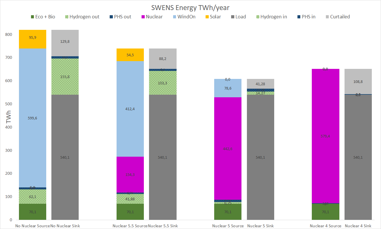
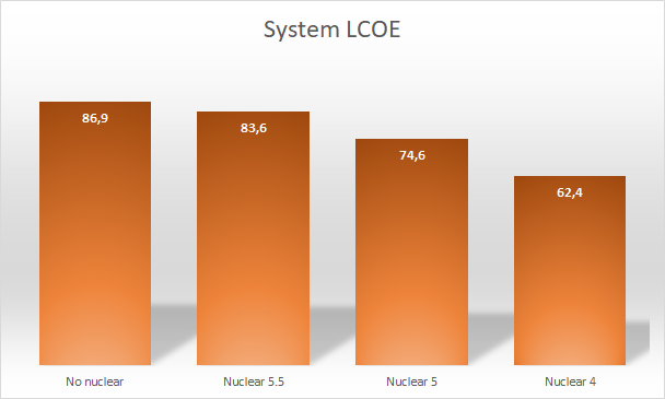
The minimum total cost is given by the Nuclear 4 case, where nuclear costs 4 GUSD/GW. The highest cost is for the No Nuclear case. Nuclear 5 and 5.5 are in between.
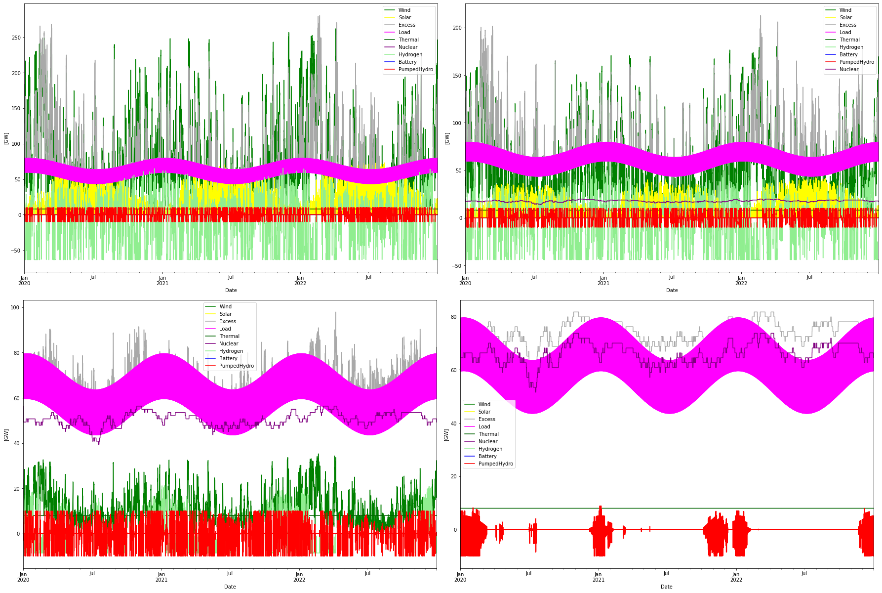
Below a graph of how the power dispatch looks for the four cases.
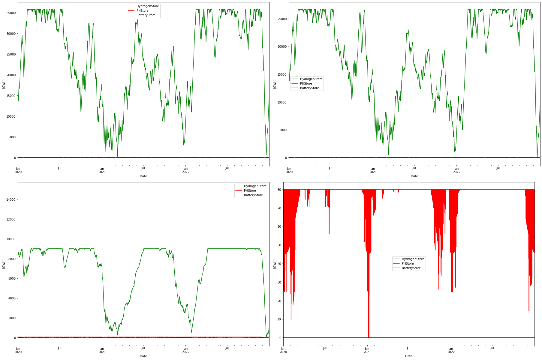
And a graph of the storage levels.
CAPEX and OPEX cost assumptions
The absolute hardest part of this work is to find a set of un-biased, consistent, and realistic numbers for future CAPEX and OPEX costs. This is more or less an impossible task, because different authors may be biased towards their preferred power sources, the cost varies in various parts of the world, the future cost development is impossible to predict etc. Anyway, we must have some costs included so here are my own estimates on wind and solar power from diverse sources. They should be “reasonable”, and since they are the same for all simulations, we can do a comparative study.
	CAPEX[GUSD]/GW(h)  OPEX[MUSD]/MW(h)/year   LCOE[USD/MWh]
WindOn   	1	           20                  37.4
WindOff	        3	           60                  67.3
Solar	        0.5	           15                  47.5
Eco	        0	            0
H2Store	        0.002 	            0
H2Elys	        0.5	           15
H2CCGT	        0.75	           15
PHStore	        0	            0
BatteryStore	0.15	            3
Nuclear 4       4                 150                  50.6
Nuclear 5       5                 200                  64.8
Nuclear 5.5     5.5               225                  71.9
The following capacity factors are used (higher than in the RQ paper):
Offshore wind power: 50%
Onshore wind power:  30%
Solar/PV power:      13%
Eco and PHS are considered “non-investible assets”, that is, they are kept as they are today. Eco is mostly biomass and hydro power, but also miscellaneous other as waste, geothermal etc. This part is simply modeled as a constant power source of 8 GW producing roughly 70 TWh per year. (See for instance this chart). Pumped Hydro Storage (PHS) is estimated as a storage type with 10 GW in and out, 80 GWh storage and roundtrip efficiency of 80%. This is an estimate of the PHS capacity today. These non-investible assets are not part of the cost calculations but contribute to the power production.
CAPEX costs for power sources are expressed in GUSD/GW installed capacity. For storage there are three cost factors. One each for charging and discharging the store, that is electrolyzers and CCGT for hydrogen stores and inverter cost for the battery store. Then there is a cost per storage unit in GUSD/GWh. For the battery inverter the same charging and discharging capacity is used, hence there are only two cost parameters for batteries.
The three nuclear cases are named “Nuclear X” where X is the over-night CAPEX cost according to the table above. Nuclear power is modelled as 40 independent reactors that have an availability given by a Markov process. The power capacity of the reactors is scaled to provide the requested total energy/power. The capacity factor for nuclear is 89.6%.
Cost for the hydrogen storage is taken from the RQ paper but added 2% OPEX cost. Also, electrolyzer and and hydrogen CCGT costs are from that paper (slightly higher OPEX on electrolyzers here).
These CAPEX and OPEX numbers are then used to provide an estimate of the System LCOE (using annualized CAPEX and OPEX costs at 6% discount rate, and the energy produced to serve the load, which is 540 TWh per year). By calculating the System LCOE in this way, all costs are internalized, and the total system costs can be compared on equal footing. Lifetime is set to 25 years for all technologies except nuclear that has 60 years and battery storage with a 15-year lifetime.
Note also that the “copper plate” assumption is used regarding the transmission network. That is, no transmission costs are calculated, it is just assumed that enough transmission is available. Including transmission would most probably favor mixes with more local production (that is, nuclear).
Also, like the RQ model, no import or export is considered. This is of course not realistic, but on the other hand, if import is allowed, a much higher degree of complexity (or arbitrariness…) is included. Import becomes a flexible power source that hides the domestic power production problems. Not using this makes the model focus on the inherent qualities of the power system and provides self-sufficiency for power supply.
Model and simulation
A time series of wind and solar power data for Germany 2020-2022 from the ENTSO-E transparency platform, together with a simulated nuclear power time series and the fixed 8 GW eco power, provides the “must-run” power sources. These are balanced, hour by hour, against the consumption (load) and against, in this order
- A battery store
- A pumped hydro store
- A hydrogen store
Like in the RQ model no import or export is allowed. Each hour can be either balanced or have an excess or deficit of power. Excess power is curtailed. Consumption is modelled as a sinusoidal load curve over the year with maximum in the winter and minimum in the summer. A daily variation is modeled, also a sinusoidal, which is added to the yearly variation curve. The load curve adds upp to 540 TWh per year.
Global and local optimization algorithms were used to find the minimum cost system that serves the load. The only constraint is that there must not be any deficit. That is, excess power can (and will) occur if it lowers the total cost, but no hour in the time series can have a deficit.
Discussion
“Nullified” power sources: Offshore wind and Batteries
In all cases or scenarios offshore wind was excluded by the optimizing algorithms. Heuristically this could be explained by the fact that the cost for offshore wind is so much higher than onshore wind, while not being sufficiently “different” from the onshore wind. There is no reason for the optimizer to add more offshore wind with similar properties as onshore wind, at a higher cost.
Batteries are also squeezed out in all calculations. This is most probably because the storage capacity (GWh) is expensive compared to the hydrogen storage capacity. Hence the hydrogen storage can be extended to “take over” the battery storage at a lower cost than building the battery store. Also, the demand model can impact. Since a “sinus/sinus” model is used for load, that is a sinusoidal for yearly variation with a sinusoidal for daily variation super-imposed, no real demand spikes are modeled. But if demand spikes with short duration occurs it is probably cheaper to build batteries that are cheap with respect to power capacity compared to CCGT power. This should be further investigated.
Removing Offshore wind and Battery storage power and capacity parameters is particularly good since optimization can work with fever parameters and then becomes stabler and faster. When finding a minimum, offshore wind and batteries are added back to ensure that the minimum is not affected by these.
Nuclear 4 case
With the cost parameters used, the Nuclear 4 case provided the minimum cost to serve the load. Interestingly all other power sources were squeezed out and using only overproduction of nuclear power gave the minimum cost! (The contribution from Eco is fixed and present in all cases, and the PHS is included all the time and not part of the cost optimizations). PHS power is used only when the demand is higher than what nuclear can produce and hence not used as much as in the other scenarios.
The minimum region of the cost function is rather flat, so there were other suggestions to build somewhat less nuclear power and instead add wind power and storage. But at the rock bottom cost-wise where the nuclear only alternative. As can be seen, quite a large curtailment is taking place for the all-nuclear alternative, which at first thought seems counter-intuitive, mainly because thinking of nuclear as a base load power form. But the alternative, to provide less nuclear and build more hydrogen storage with electrolyzers and turbins at low utilization and efficiency always become more expensive than overproducing nuclear in this case.
The Nuclear 4 case has 28% lower cost than the No Nuclear case.
Nuclear 5 case
In the intermediate Nuclear 5 case (CAPEX 5 GUSD/GW for nuclear) the optimal mix as seen in the figure above is 440 TWh (from 56 GW installed nuclear power) and 80 TWh onshore wind power (30 GW installed) with a hydrogen storage of 9 TWh (input power, corresponding to 6 TWh H2 LHV) and 9 GW / 21 GW electrolyzers and H2 CCGT capacities. We can also see here that the curtailed energy is actually lower in this case than in the Nuclear 4 case. Some of the excess energy goes into the PHS and hydrogen stores, but even with this considered the curtailment is lower.
Also note that not only offshore wind, but also solar/PV is nullified in this scenario. The Nuclear 5 case has 14% lower cost than the No Nuclear case.
Nuclear 5.5 case
In the Nuclear 5.5 case it is seen that the optimizer prefers onshore wind as power source. Solar is entering the optimal solution and nuclear still provides a good share of the power. 4% lower cost than No Nuclear.
No Nuclear case
This case should be quite similar to the RQ case and indeed it is. A difference is that the optimizer has squeezed out offshore wind from the power mix. This can be attributed to the much higher cost for offshore wind in this work. Other differences can be accounted for by the differences in weather patterns (2020->2021->2022 had a strong variation in wind/solar production, 180->160->180 TWh), and that here 40% is used as round-trip efficiency for the power->hydrogen->power cycle, instead of 50% that is used by RQ.
The System LCOE becomes 76 USD/MWh, which can be compared to the 80 USD/MWh concluded by RQ. But here a smaller 36 TWh (24 TWh H2 LHV) store is used, only covering the 2020-2022 weather pattern. If the store is extended to 54.8 TWh (LHV) that RQ concludes as the worst case, the system LCOE increases to 89 USD/MWh.
General notes
Hydrogen storage and power generation increases with increased VRE penetration just as expected. Note that the hydrogen storage capacity range 9 to 36 TWh is measured in input energy terms. In H2 LLV calorific energy value terms they correspond to 6 – 24 TWh. This should be compared to the worst-case value of 54.8 TWh that RQ concluded was needed to handle the lowest wind conditions during the 37 years they studied. With more nuclear power in the mix also this worst-case storage size will be smaller, but it is not clear by how much.
In the No Nuclear case a high degree of excess energy is produced to reduce the storage costs. The excess is higher here than in the RQ paper, this is probably because here the capacity factors for the RE sources are higher, making it cheaper to produce more energy.
Now it should be noted that the excess energy could be used to, for example, export or for hydrogen production (for industrial use). However, it is likely that the export price of the excess energy would be quite low (or even negative). Also, it is hard to utilize the excess power spikes that can be very strong, thus a high capacity of the export lines is needed to harvest this excess energy, and with a low utilization factor. The same applies to hydrogen production. Usage of excess energy for hydrogen production for industrial purposes results in an exceedingly high cost for hydrogen. For the No Nuclear case, 210 GW of extra electrolysis capacity is needed to utilize all 130 TWh of excess energy. This would yield a utilization factor of 7% of the electrolyzers. On the other hand, in the Nuclear 4 case, with a “steady” overproduction, 108 TWh of hydrogen could be produced with 34 GW of electrolyzers, then working at a 36% utilization factor.
It should also be noted that the cost for the transmission network is not included. That cost will increase with higher penetration of variable renewable power production.