
Bengt J. Olsson
Twitter: @bengtxyz
LinkedIn: beos
What if Europe had a perfectly connected power system in 2050? With no transmission network limitations. This will be a long post, juggling large numbers, and with many assumptions that will make this investigation rather speculative. Anyway, you have been warned! What I have done is to use Energy Charts combined data for EU27 and added Norway (because of their large energy storage in form of hydro reservoirs), removed fossil fuels and replaced with optimized amounts of RE and nuclear power, to cover the electricity and hydrogen needs for 2050. The system is considered to be perfectly connected with no import and export. An estimation is also done on the contribution of Network and System overhead costs to the total system cost.
The final System LCOE is estimated to be between 79 – 91 EUR/MWh depending on scenario.
Introduction
Model
Simulations
– Scenario 1: Unrestricted optimal generation
– Scenario 2: Restricted onshore wind power (1300 TWh)
– Scenario 3: No nuclear power
Summary
Introduction
Loosely based on the “EU Fit for 55” (FF55) energy scenario, three power system alternatives for EU27 + NO are presented. According to the FF55 scenario, EU will consume roughly 6000 TWh by 2050, doubling from today’s 3000 TWh consumption. Out of these 6000, more than 1000 TWh will be used for Power to X, which essentially is hydrogen production. The non-hydrogen increase in consumption is due to many things, but largely because of increased electrification in heating (for example heat pumps), industrial processes (for example iron ore production, green fertilizers), as well as transportation.
This increased consumption will need a large build-out of the European power system. This post investigates the most cost-effective ways to meet the 2050 demands from a balance model perspective. The balance model has many simplifications but provides a good overview of what is needed and how it is spent. Maybe the largest simplification is that transmission and system costs are not included in the model. Like in many other models, a “copper-plate” transmission medium is assumed, that is, there are no limitations caused by transmission. This would be an ideal system, especially for a system based largely on renewable energy (RE). For such a system a high degree of transmission is needed for transport of energy between different parts of Europe, depending on the weather conditions. In a real system, transmission bottlenecks will of course limit how power can be produced and consumed.
Three scenarios will be explored. The first is produced using an unlimited cost optimization. This means that the model produces the system with lowest total cost given the input cost parameters. This scenario will produce a lot of onshore wind power, since it is the most cost optimal power source given its combination of low CAPEX/OPEX costs and a relatively high assumed capacity factor of 35%.
The second scenario is the same as the first but puts a limit on the amount of onshore wind power production. This limit is set to 1300 TWh in 2050 and corresponds to a continuation of the linear growth we see in the EU27 + NO installed onshore wind power data from Energy Charts (EC).
The third scenario looks at a scenario with no nuclear power.
Model
Data input to the model comes mainly from two sources: Energy Charts for hourly power production and consumption data, and from this very thorough and interesting report from Eurelectric for future electricity and hydrogen needs. The model includes EU27 + Norway. Norway is included since it provides a large part of the flexible hydro power that is needed for balancing, and will be even more important when flexible fossil power sources are terminated. The Eurelectric report handles EU27 + GB, so the match is not perfect but good enough for this relatively coarse model.
Data normalization and scaling
The approach here is to use the Energy Charts (EC) hourly data for EU27 + Norway, for the three years 2021-2023, exclude all fossil power sources, normalize the data, and increase the load to the levels of FF55 in 2040. All power sources except Onshore/Offshore wind, Solar, and Nuclear power are held at the same level as today. This means that categories hydro run-of-river, biomass and pumped hydro as well as geothermal and other today available (non-fossil) power sources are kept as is in the data and constitute “must-run” power. Likewise, the EC load data is kept as is but scaled to the future requested level (pumped hydro consumption is added to the load as well). Normalization is done by scaling each power source to have three years with similar levels for all the power sources. An exception is that the nuclear levels for 2022 are kept at a lower level to include the effect of systematic failures like we saw in France 2022. For onshore/offshore wind power the data has also been scaled in such a way that relatively more power is produced at lower power levels (linearly from 10% more at zero levels to 0% more at max levels), simulating a better low-wind efficiency in future wind power technology.
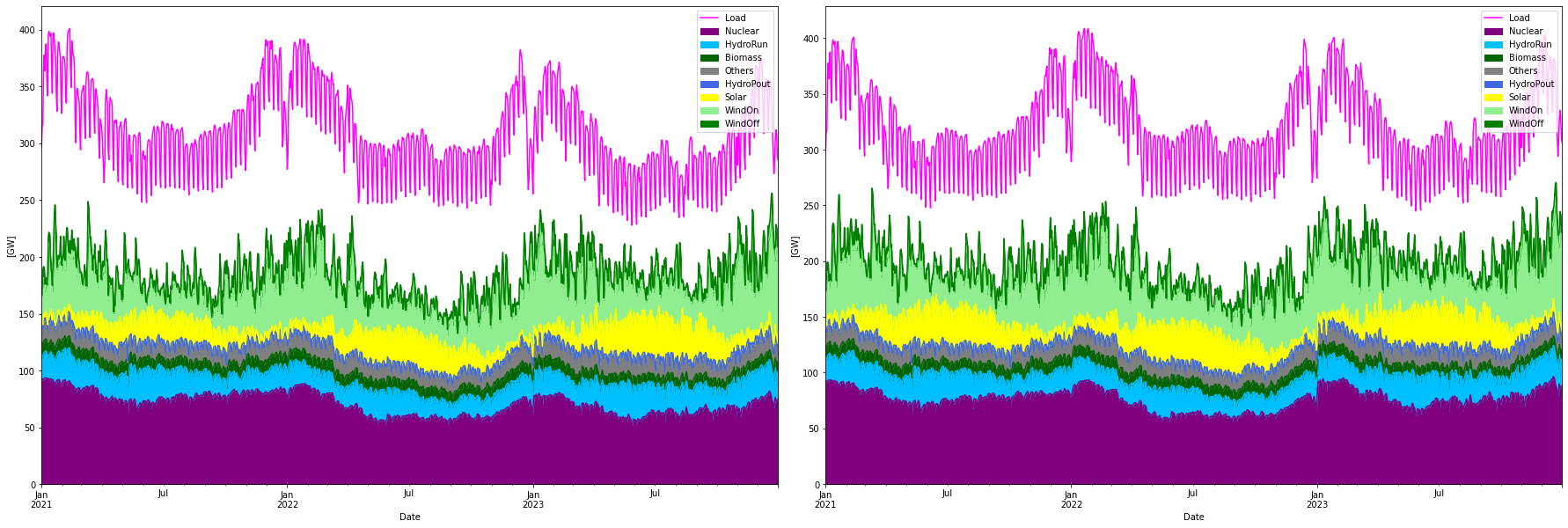
There are mainly three features in the normalization: 1. Solar for 2021/2022 increased to 2023 levels. 2. Nuclear normalized to 85/75/85% capacity factor for 2021-2023. 3. Load for 2022/2023 increased to 2021 levels. Onshore wind is also normalized, but hardly visible. All in all this normalization provides three years with relatively stable production and consumption but with the real statistical variation of the three years.
During the simulation the levels of on/offshore wind, solar and nuclear power will be scaled to provide the requested yearly energy production in TWh. These energy values are parameters to be optimized. Nominal load (before hydrogen production) is scaled with a fix scale factor to get to the predetermined (from Eurelectric FF55 scenario for 2050, 4856 TWh per year).
Energy stores
Two energy stores are used. One for hydro reservoir power with a capacity of 140 TWh and with an assumed output capacity of 0 – 70 GW. The inflow to this store is modeled empirically to simulate the seasonal inflow in Norway’s and Sweden’s large reservoirs and a constant inflow representing the rest of EU. The total inflow per annum is set to 240 TWh (following EC data).
The hydrogen energy store is modelled based on the Eurelectric method and data, with some smaller adjustments. The report states that the Power-to-X industry needs 1672 TWh of hydrogen in 2050. And that 923 TWh is imported from outside Europe. The rest + hydrogen for hydrogen CCGT power plants will be produced by electrolyzers within Europe.
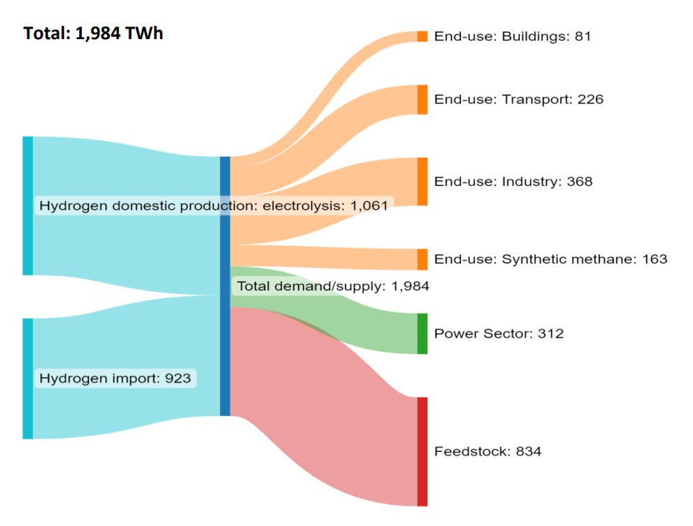
1984-312 = 1672 TWh (LHV), and import capacity is 923/0.75/8.76 = 140.5 GW.
Recalculating from hydrogen LHV to the corresponding electrical energy to produce the hydrogen, with a 75% electrolyzer efficiency, the following flows according to the figure below are acquired. Out of Store: 2230/8.76 = 254.6 GW for the delivered hydrogen and an import corresponding to 140.5 GW in electric power. Note that in this model, the import will be less than 923 TWh (LHV) since it will not be possible to import when the store is full. The dynamic hydrogen production using electrolyzers will balance the production, and the store will make sure that 254.6 (2230/8.76) GW worth of hydrogen always can be delivered for Power to X customers, and as well to be combusted in hydrogen CCGTs when needed. The hydrogen balance is presented in each simulation.
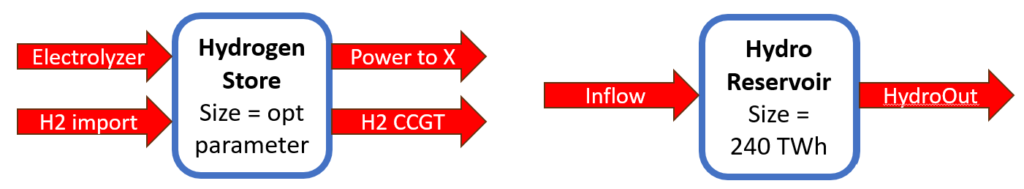
H2 import: 140.5 GW (unless store is full)
Power to X: 2230/8.76 = 254.6 GW
Electrolyzer and H2 CCGT flows are dynamic
The imported hydrogen is assigned a cost of $1.5 per kg, see cost section below how this translates into power terms. The import cost is included in the total system cost calculation.
Optimization
The amount of Onshore/Offshore wind, Solar, and Nuclear power are optimization parameters. So are the size of the hydrogen store, the electrolyzer capacity, and the hydrogen CCGT capacity. All in all 7 optimization parameters. Optimization is performed by minimizing the total annualized cost of the system, given a number of cost parameters and subject to the two conditions that no deficit should occur and that the hydro reservoir power generation should be less than 240 TWh. (Actually some deficit is also allowed since it would be to costly to cover all deficits. But the total deficit in the simulations is well below 0.5 TWh per year, and in practice these would be managed by additional flexibility mechanisms, such as battery store or consumption flex due to high spot price).
For the power sources the cost parameters are taken from the latest “long term market analysis” by the Swedish TSO Svenska Kraftnät (“LMA2024“), and are given in the simulation printouts along with the estimated LCOE for each power source. Most interesting is the System LCOE here defined as the total annualized cost divided by the annual energy produced that meets the consumption. The System LCOE is interesting since it internalizes all balancing, or “firming” costs that are needed when production capacity does not match demand. It is this System LCOE that is minimized in the optimization.
Balancing
For balancing, three mechanisms are used
- Hydro reservoir power (increase supply)
- Hydrogen production flexibility (increase/decrease demand)
- Hydrogen CCGT power (increase supply)
Balancing is a little bit tricky since the dispatch of balancing power should be based on market pricing principles, which are very non-linear and difficult to simulate. Here, a simpler approach is used.
- For “negative” balancing, that is, production is higher than nominal consumption, the only available mechanism is to produce more hydrogen (i.e. increasing demand), so that is simple.
- For “positive” balancing there are there possible sources. Supply more hydro reservoir power, decrease the demand by producing less hydrogen and finally, supply more power in the form of hydrogen CCGT turbines. The dispatch order of these power sources is set as
- If the relative fill level of the hydrogen store > two times the relative fill level of the hydro reservoir store, then dispatch
First: Hydrogen production flexibility (decrease demand)
Second: Hydro reservoir power (increase supply)
Else
Dispatch as above but in reverse order - Third: Dispatch hydrogen CCGT power (increase supply)
That is, hydro reservoir power or hydrogen production flexibility will always be dispatched before hydrogen CCGT since the latter will be the most expensive way to supply balancing power. The conditioned dispatch of the first two stored sources will have in effect that store levels are managed to be as high as possible, thus maintaining the largest possible reserve at all times. The factor two times is an empirical factor that was needed to not spill too much water. No rate limits are imposed on the balancing powers.
Batteries are not included, because at the cost points used, they would compete with the H2 CCGT and most likely loose to these due to their cost in combination with their low storage capacity. That is, even if a 2 hour battery is cheaper per GW than a H2 CCGT, if it runs out before the deficit is covered, then the H2 CCGT has to dispatch to cover the rest of the deficit. Then it is in total more cost effective to only have and use the H2 CCGT. I have seen this in other simulations as well. Batteries are good for local peak-shaving and for handling disturbances and other system services, but not cost effective enough for bulk energy balancing on national scale. Since we don’t model local bottlenecks etc. here there is no use for batteries.
No import/export (other than the hydrogen import) is allowed in the model. Europe should be self-sufficient with respect to energy.
Cost and other input data
Costs used for the simulations are the following. For wind/solar/nuclear/CCGT costs are taken from the Swedish TSO Svenska Kraftnät (SvK) report “Långsiktig marknadsanalys” for 2045. For offshore wind power, the lower cost option is used. For Solar an intermediate value between roof-top solar and solar parks is used. Also for nuclear the intermediate value between large and SMR nuclear plants was used. Hydrogen storage and Electrolyzers are my estimations. The following costs are used
| Component | CAPEX (overnight cost) | OPEX (yearly cost) | Lifetime | Capacity factor | Discount rate | LCOE |
|---|---|---|---|---|---|---|
| Solar/PV power | 0.5 BEUR / GW | 8.3 MEUR/ GW | 30 y | 15% | 6% | 34.0 EUR/MWh |
| Onshore Wind power | 1.03 BEUR/ GW | 30 MEUR / GW | 25 y | 35% | 6% | 36.1 EUR/MWh |
| Offshore Wind power | 1.425 BEUR / GW | 69.2 MEUR / GW | 25 y | 50% | 6% | 41.3 EUR/MWh |
| Nuclear power | 4.4 BEUR / GW | 88.4 MEUR / GW | 60 y | 85% | 6% | 48.4 EUR/MWh |
| Hydrogen Storage | 1 BEUR / TWh | 20 MEUR / TWh | 40 y | N/A | 6% | N/A |
| Electrolyzer capacity | 0.5 BEUR / GW | 15 MEUR / GW | 25 y | N/A | 6% | N/A |
| Hydrogen CCGT | 0.549 BEUR / GW | 12.5 MEUR / GW | 40 y | N/A | 6% | N/A |
| Hydrogen import | N/A | 45.1 MEUR / TWh (LHV) 33.8 MEUR / TWh (1.5 EUR / kg) | N/A | N/A | N/A | 33.8 EUR/MWh |
Hydrogen import costs (given by SvK as 45.1 EUR/MWh, corresponding to 1.5 EUR/kg H2), is scaled by the assumed electrolyzer efficiency, 75%, to a corresponding “electricty import” value of 33.8 EUR/MWh since the hydrogen energy amount is measured in terms of energy used to produce it instead of its LHV. That is a flow of 1 GW of hydrogen actually means a flow of 0.75 GWh/h hydrogen measured by its LHV. (BTW, this import price is lower than the LCOE of any produced power within EU).
Very important are of course the capacity factor estimations. These will have a direct influence on the LCOE and hence on the optimization results. Using single capacity factors is a weakness of this model, since these will vary significantly over Europe. Thus the values are estimated over-all average capacity factors for the whole Europe. The following values were used:
Solar: 15%
Onshore Wind: 35%
Offshore Wind: 50%
Nuclear: 85%
Simulations
Several simulation steps were performed to find the cost optimal solutions. Given the non-linear character of the optimization problem, it is somewhat of “crafts-work” to find the global minimum and avoid winding up in local minima. The method used here is to, in a first step, reduce the time resolution and resample the data to days instead of hour, thus reducing the data amount with a factor 24. This reduced data set is the used together with a “differential evolution” optimization algorithm that is good at finding global minima (but consumes tremendous cpu resources…). When the global minimum was found in this way, the solution is used as input to an optimization using the full set of hourly data, using a Nelder-Mead algorithm. There are many close local minima in the cost hyper-surface but they are grouped together in distinct areas, one area for each scenario, of the cost space.
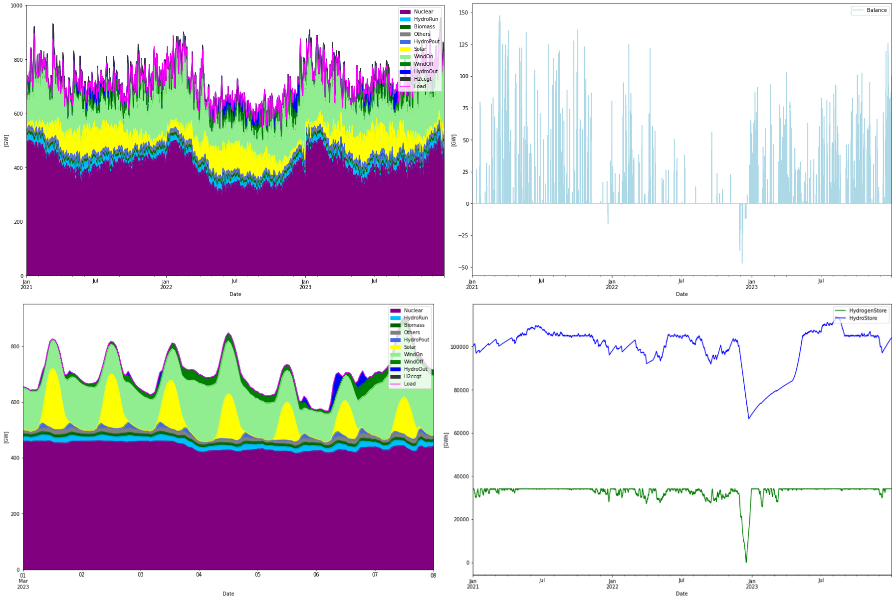
Scenario 1. Unrestricted optimization case
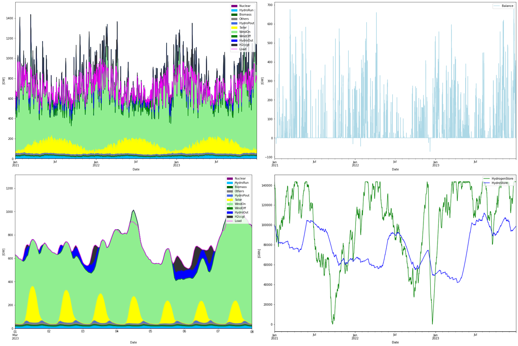
In this case all seven parameters (Yearly energy production for solar/onshore/offshore/nuclear power, hydrogen store size, electrolyzer and hydrogen CCGT capacity) were used as optimization parameters. The result of the optimization is shown below.
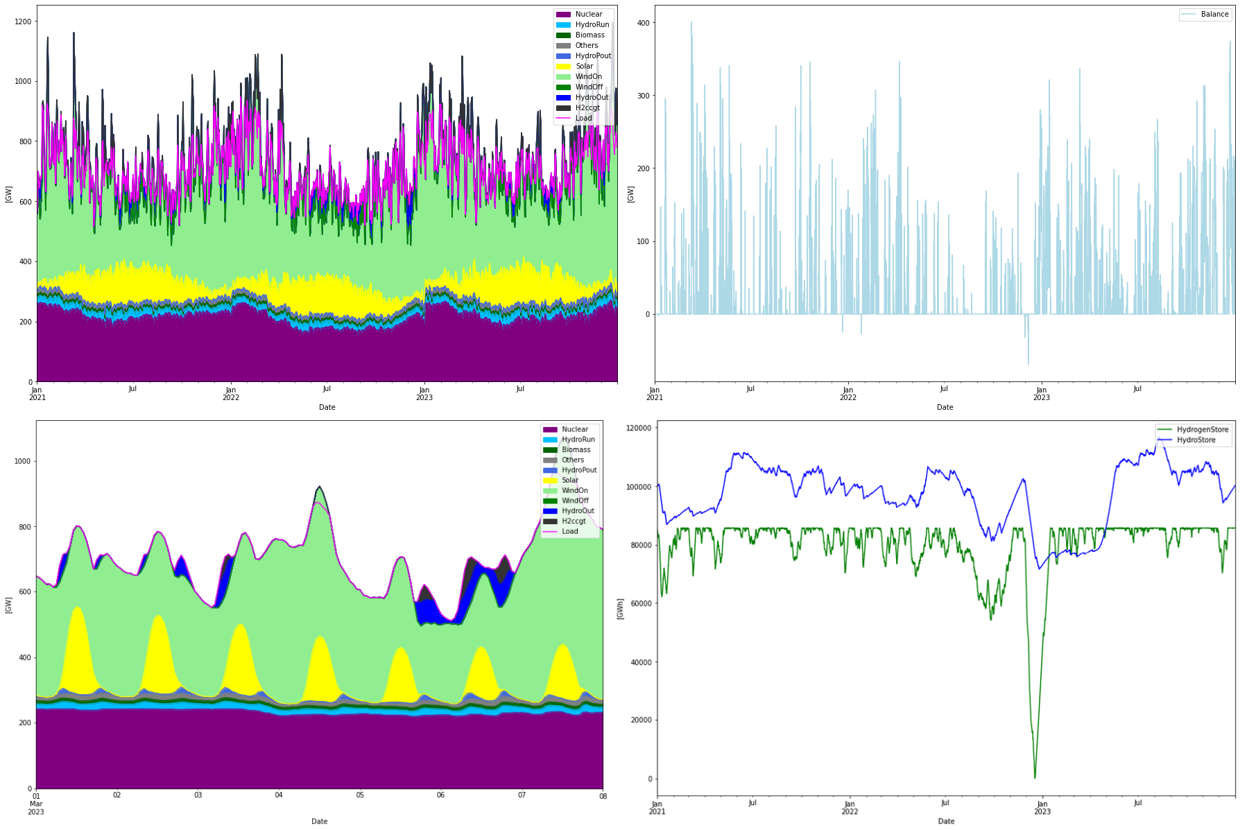
           Installed Capacity Unit  TWh/year  CAPEX/GW(h)  OPEX/MW(h)/y   CRF  Tot CAPEX  Tot OPEX  Ann Cost    LCOE
WindOn              1028.170   GW  3152.369        1.030        30.000 0.078   1059.015    30.845   113.688  36.064
WindOff                0.000   GW     0.000        1.425        69.200 0.078      0.000     0.000     0.000     NaN
Solar                515.708   GW   677.640        0.500         8.300 0.073    257.854     4.280    23.013  33.961
Nuclear              252.466   GW  1879.863        4.400        88.360 0.062   1110.851    22.308    91.043  48.430
H2Store            85758.000  GWh     0.000        0.001         0.020 0.066     85.758     1.715     7.415     inf
H2Elys               254.658   GW     0.000        0.500        15.000 0.078    127.329     3.820    13.780     inf
H2ccgt               126.916   GW    16.332        0.549        12.500 0.066     69.677     1.586     6.217 380.679
H2import               1.000  N/A   927.727        0.000        33.825 0.060      0.000    31.380    31.380  33.825

Total over-night cost         2710.5 BEUR
Total yearly OPEX costs         95.9 BEUR
Annualized cost             286.5370 BEUR
System LCOE                  59.3816 EUR/MWh
Yearly energy balance
---------------------
Nuclear       :  1880 TWh/a (29.5%)
HydroRun      :   189 TWh/a ( 3.0%)
Biomass       :    82 TWh/a ( 1.3%)
Others        :   103 TWh/a ( 1.6%)
HydroPout     :    40 TWh/a ( 0.6%)
Solar         :   678 TWh/a (10.6%)
WindOn        :  3152 TWh/a (49.4%)
WindOff       :     0 TWh/a ( 0.0%)
HydroOut      :   240 TWh/a ( 3.8%)
H2ccgt        :    16 TWh/a ( 0.3%)
HydroPin      :   -41 TWh/a
Load          : -6134 TWh/a

Total Produced:  6379 TWh/a
Total Consumed: -6174 TWh/a
---------------
    Difference:   205 TWh/a

Deficit       :     0 TWh/a
Curtailed     :  -205 TWh/a
       Balance:    -0 TWh/a
Yearly H2 store balance
-----------------------
Total produced:  1349 TWh/a
Total imported:   928 TWh/a
Total delivered: 2230 TWh/a
Total combusted:   47 TWh/a
Store change:       0 TWh/a
       Balance:    -0 TWh/a

Yearly Hydro store balance
--------------------------
Total inflow:   239.9 TWh/a
Total outflow:  239.8 TWh/a
Store change:     0.1 TWh/a
       Balance:   0.0 TWh/a
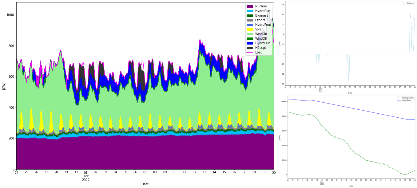
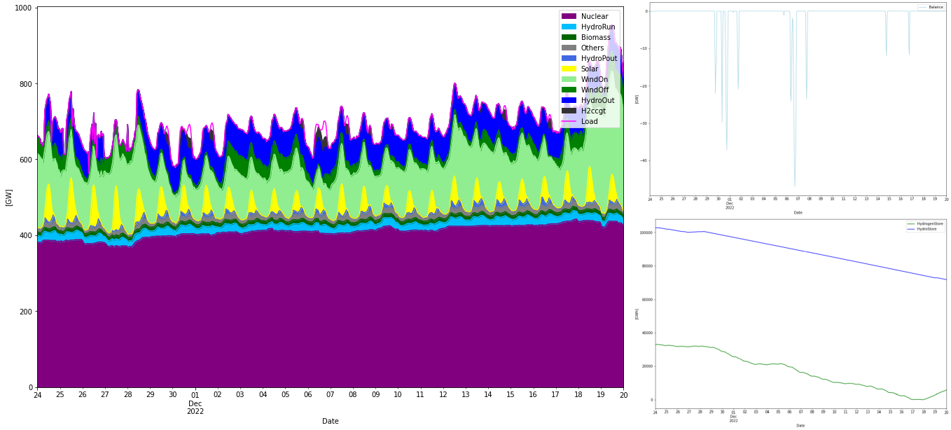
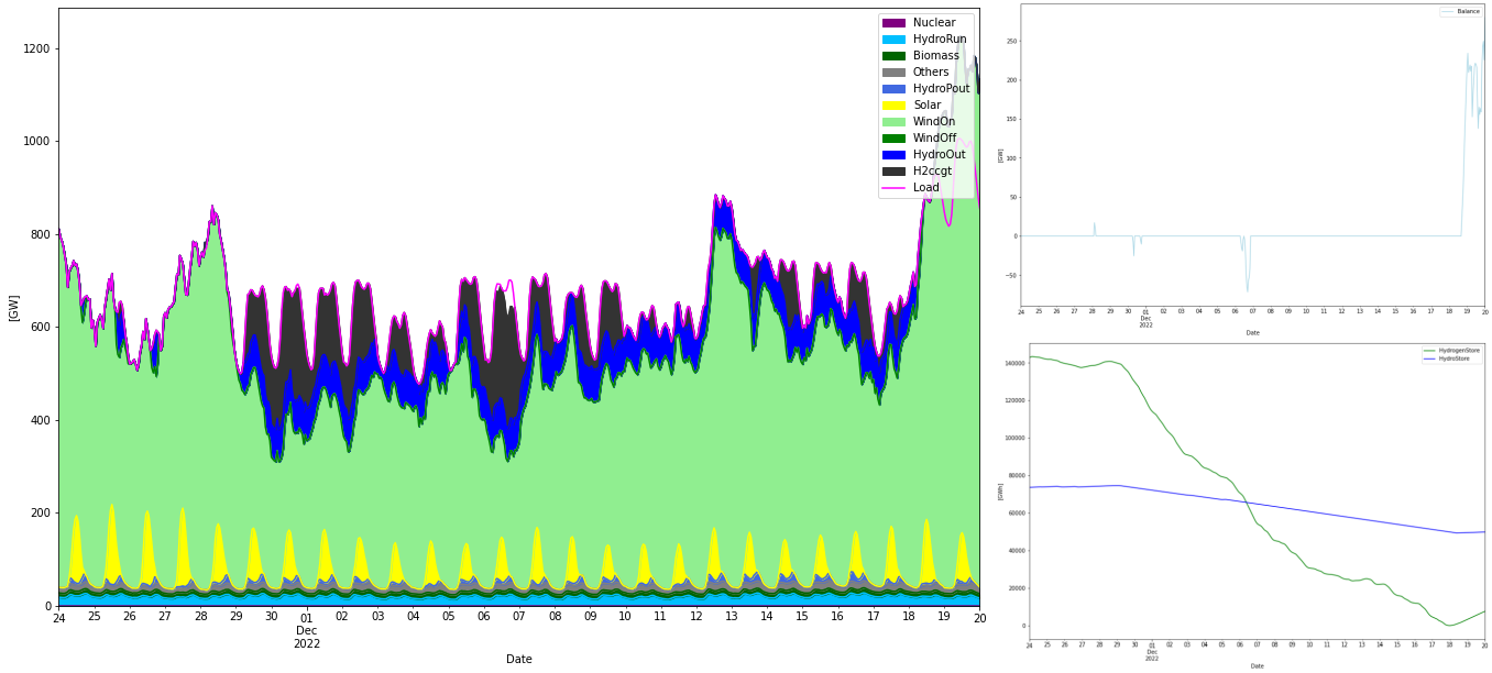
As can be seen in the storage graph, the most difficult period to handle is in December 2022 so let’s expand this period:
Scenario 2. 1300 TWh limit on onshore wind power
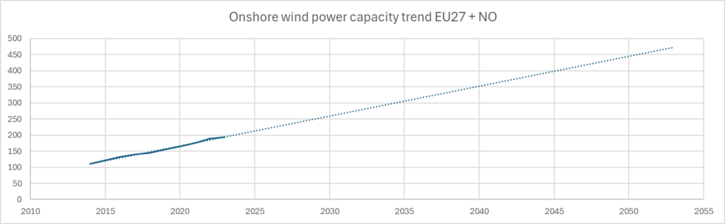
In this simulation we only vary six parameters, the onshore wind power production is held at 1300 TWh/year. This value roughly corresponds to a development where the linear growth in installed capacity that we have seen from 2014 to 2023 (according to EC) continues. That is, resistance in building onshore wind power for various reasons hampers the higher growth rate that is needed in the unrestricted scenario above. The optimization results for this scenario is seen below
           Installed Capacity Unit  TWh/year  CAPEX/GW(h)  OPEX/MW(h)/y   CRF  Tot CAPEX  Tot OPEX  Ann Cost     LCOE
WindOn               424.005   GW  1300.000        1.030        30.000 0.078    436.725    12.720    46.884   36.064
WindOff               49.554   GW   217.046        1.425        69.200 0.078     70.614     3.429     8.953   41.250
Solar                416.807   GW   547.684        0.500         8.300 0.073    208.403     3.459    18.600   33.961
Nuclear              482.324   GW  3591.383        4.400        88.360 0.062   2122.225    42.618   173.932   48.430
H2Store            34133.600  GWh     0.000        0.001         0.020 0.066     34.134     0.683     2.951      inf
H2Elys               254.594   GW     0.000        0.500        15.000 0.078    127.297     3.819    13.777      inf
H2ccgt                27.303   GW     0.854        0.549        12.500 0.066     14.989     0.341     1.337 1565.538
H2import               1.000  N/A   790.620        0.000        33.825 0.060      0.000    26.743    26.743   33.825

Total over-night cost         3014.4 BEUR
Total yearly OPEX costs         93.8 BEUR
Annualized cost             293.1772 BEUR
System LCOE                  60.7577 EUR/MWh
Yearly energy balance
---------------------
Nuclear       :  3591 TWh/a (56.9%)
HydroRun      :   189 TWh/a ( 3.0%)
Biomass       :    82 TWh/a ( 1.3%)
Others        :   103 TWh/a ( 1.6%)
HydroPout     :    40 TWh/a ( 0.6%)
Solar         :   548 TWh/a ( 8.7%)
WindOn        :  1300 TWh/a (20.6%)
WindOff       :   217 TWh/a ( 3.4%)
HydroOut      :   239 TWh/a ( 3.8%)
H2ccgt        :     1 TWh/a ( 0.0%)
HydroPin      :   -41 TWh/a
Load          : -6227 TWh/a

Total Produced:  6309 TWh/a
Total Consumed: -6267 TWh/a
---------------
    Difference:    42 TWh/a

Deficit       :     0 TWh/a
Curtailed     :   -42 TWh/a
       Balance:     0 TWh/a
Yearly H2 store balance
-----------------------
Total produced:  1442 TWh/a
Total imported:   791 TWh/a
Total delivered: 2230 TWh/a
Total combusted:    2 TWh/a
Store change:       0 TWh/a
       Balance:    -0 TWh/a

Yearly Hydro store balance
--------------------------
Total inflow:   239.9 TWh/a
Total outflow:  238.6 TWh/a
Store change:     1.3 TWh/a
       Balance:   0.0 TWh/a
Scenario 3. No nuclear power
I this scenario nuclear power is completely eliminated and replaced with only RE power.
           Installed Capacity Unit  TWh/year  CAPEX/GW(h)  OPEX/MW(h)/y   CRF  Tot CAPEX  Tot OPEX  Ann Cost    LCOE
WindOn              1660.302   GW  5090.487        1.030        30.000 0.078   1710.111    49.809   183.585  36.064
WindOff                0.000   GW     0.000        1.425        69.200 0.078      0.000     0.000     0.000     NaN
Solar                603.851   GW   793.460        0.500         8.300 0.073    301.925     5.012    26.947  33.961
Nuclear                0.000   GW     0.000        4.400        88.360 0.062      0.000     0.000     0.000     NaN
H2Store           143366.400  GWh     0.000        0.001         0.020 0.066    143.366     2.867    12.396     inf
H2Elys               293.755   GW     0.000        0.500        15.000 0.078    146.878     4.406    15.896     inf
H2ccgt               240.365   GW    85.259        0.549        12.500 0.066    131.960     3.005    11.775 138.106
H2import               1.000  N/A  1113.180        0.000        33.825 0.060      0.000    37.653    37.653  33.825

Total over-night cost         2434.2 BEUR
Total yearly OPEX costs        102.8 BEUR
Annualized cost             288.2519 BEUR
System LCOE                  59.7370 EUR/MWh
Yearly energy balance
---------------------
Nuclear       :     0 TWh/a ( 0.0%)
HydroRun      :   189 TWh/a ( 2.9%)
Biomass       :    82 TWh/a ( 1.2%)
Others        :   103 TWh/a ( 1.5%)
HydroPout     :    40 TWh/a ( 0.6%)
Solar         :   793 TWh/a (12.0%)
WindOn        :  5090 TWh/a (76.9%)
WindOff       :     0 TWh/a ( 0.0%)
HydroOut      :   240 TWh/a ( 3.6%)
H2ccgt        :    85 TWh/a ( 1.3%)
HydroPin      :   -41 TWh/a
Load          : -6145 TWh/a

Total Produced:  6623 TWh/a
Total Consumed: -6186 TWh/a
---------------
    Difference:   437 TWh/a

Deficit       :     0 TWh/a
Curtailed     :  -437 TWh/a
       Balance:    -0 TWh/a
Yearly H2 store balance
-----------------------
Total produced:  1360 TWh/a
Total imported:  1113 TWh/a
Total delivered: 2230 TWh/a
Total combusted:  244 TWh/a
Store change:       0 TWh/a
       Balance:    -0 TWh/a

Yearly Hydro store balance
--------------------------
Total inflow:   239.9 TWh/a
Total outflow:  240.4 TWh/a
Store change:    -0.4 TWh/a
       Balance:  -0.0 TWh/a
Summary
First of all it must be emphasized that this is not an academic or scientific work, it is a blog post using a model that is very simplified. For example no network limitations are considered, only three years of statistics, costs are modelled such like the whole system was built-up over one night in 2050, dispatch merit order is more or less empirically decided etc. The work and results should just be considered for what they are, my own experiments with power system model that trades accuracy for simplicity. With this said I think it still provides some interesting insights and rough estimation of key numbers for the three scenarios.
The three scenarios investigated are:
- Unrestricted optimization of all seven parameters (Yearly energy production for solar/onshore/offshore/nuclear power, hydrogen store size, electrolyzer and hydrogen CCGT capacity)
- Restricted onshore wind power at 1300 TWh/y and optimizing the remaining 6 parameters.
- No nuclear power and optimizing the remaining 6 parameters.
The power mixes and hydrogen parameters in the three cases were:
| Scenario | Onshore wind power (TWh/a) | Offshore wind power (TWh/a) | Solar/PV power (TWh/a) | Nuclear power (TWh/a) | Hydrogen Store Size (TWh) | Electrolyzer capacity (GW) | Hydrogen CCGT capacity (GW) | System LCOE (EUR/MWh) |
|---|---|---|---|---|---|---|---|---|
| Unrestricted | 3152 | 0 | 678 | 1880 | 86 | 255 | 127 | 59.4 |
| Restricted onshore wind power | 1300 | 217 | 548 | 3591 | 34 | 255 | 27 | 60.8 |
| No nuclear power | 5090 | 0 | 793 | 0 | 143 | 294 | 240 | 59.7 |
In general, the assumption of total connectedness provides an averaging of dispatch over Europe. All power sources benefit from this averaging, but probably most RE power sources. Thus the “connectedness” property is also more important for RE power, and will cost more to implement, as discussed below.
Offshore wind power is more or less eliminated in the optimization, except when the amount of onshore wind power is restricted. I interpret this as the offshore wind being too similar in behavior to onshore wind, but more expensive to produce. This favors more onshore wind power. When onshore wind power is restricted to 1300 TWh, almost all the difference to its unrestricted level, become nuclear power. We can even see a small decline in the solar energy production. Could this be an effect of that there is too little wind power to “balance” the solar power since they should behave rather complementary versus each other?
The System LCOE for all scenarios is essentially the same, given the inherent error margin. Considering that about 10% of the energy is produced by the “un-investable” resources (hydro, biomass, geothermal and others), why the real system LCOE must be adjusted. Let’s assume the LCOE for the un-investable resources are 50 EUR/MWh (mostly amortized assets, but biomass have fuel costs), then the System LCOE would increase from 60 EUR/MWh to about 65 EUR/MWh.
The conclusion from the above is that it doesn’t really matter which generation we have, we get about the same “Generation System LCOE” cost of about 65 EUR/MWh. But what will be the tie-breaker then? I would say that this is Network and System overhead (NSOH) costs. Unfortunately it is very hard to find any data on levelized costs of transmission and distribution networks. By scanning on-line from various sources I would provide a span like 20% – 40% on top of the levelized generation costs. Lower region for the scenarios with much nuclear and higher region for the RE rich scenarios. This because nuclear can be built close to consumption centers and inherently provides many system utilities. And oppositely for RE rich scenarios. If we can assume this (very speculative) hypothesis and assign the following NSOH to the different scenarios, we would end up with the following finals System LCOE for the scenarios
| Scenario | Generation System LCOE | Assumed Network & System Overhead | Total System LCOE |
|---|---|---|---|
| Unrestricted optimal generation | 64 EUR/MWh | 30% | 83 EUR/MWh |
| Restricted onshore wind – nuclear rich | 66 EUR/MWh | 20% | 79 EUR/MWh |
| No nuclear – RE rich | 65 EUR/MWh | 40% | 91 EUR/MWh |
Another difference between the scenarios is their use of hydrogen flexibility. While all scenarios heavily utilizes hydrogen production flexibility (which is a good thing, since this have a very high efficiency), there is a strong difference in use of hydrogen CCGT flexibility (which is a bad thing). As predicted, the no nuclear – RE rich scenario combusts most hydrogen, 244 TWh/a (or in LHV terms, 183 TWh/a), while nuclear rich scenario only consumed 2 TWh/a and only uses 27 GW of CCGT capacity. The latter consumption could probably be replaced altogether by batteries and demand response, while this is not an option for the RE rich scenarios. This would further simplify the power systems. (I have seen similar results in an experiment with a future German power system fueled by either only offshore wind power or only nuclear power).
Hydrogen production flexibility in itself is great flexibility resource. In this case the nominal electrolyzer capacity is 114 GW, meaning that these 114.1 GW + 140.5GW from import together provides the 254.6 GW that should continually be delivered. With electrolyzer capacity between 250 – 300 GW for the scenarios it means that can provide positive flex “power” up to 114 GW (to counteract deficits), and about 140-190 GW in negative flex “power” to use power that would otherwise be curtailed. But it is only applicable if there is this large external need for hydrogen, and that sufficient hydrogen storage is available.