
Bengt J. Olsson
Twitter: @bengtxyz
LinkedIn: beos
Background
The model
Simulations
Discussion and Conclusions
Update: Nuclear-only alternative
Hydrogen storage in Denmark
Background
Denmark has plans to massively build out wind and solar power and also to produce hydrogen for PtX purposes. Here is a simple model and simulation of how such a power system could behave under three years, based on wind and solar statistics for 2020-2022. The scenario is loosely based on “Analyseforudsætninger til Energinet 2023 (AF23)” which outlines the Danish power system development to 2050.
Most important is that consumption in 2040 can roughly be described as being 76 TWh “normal” consumption and 89 TWh consumption for flexible hydrogen production. The normal consumption includes new consumption types such as electric heating, electrified transport, and data centers. However, for this model, they are treated as normal or classic consumption (since the major flexible mechanism is to move consumption from day to night, which is easily modeled by just shrinking the day/night variation of consumption).
On the production side, a large expansion is projected, especially in offshore wind and solar power. Using the projections of AF23 as limits, onshore wind power is limited to 6.5 GW by 2040, and offshore wind power is limited to a max of 29.3 GW. Solar is limited to a max of 32.2 GW. Thermal power will decrease but a substantial part will still be used since it comes from combined heat and power plants. Here this part is modeled as a fixed dispatch varying with the seasonal temperature variation. Thermal power includes (and will mainly use) biopower. Condensing biopower plants could be used for balancing, but it would be a small part and is not included in this model.
For balancing there are two possible sources. Import/export is one and the second is hydrogen production flexibility. That is to increase or decrease the power used for producing green hydrogen with electrolyzers. The projected value of 17.83 GW electrolyzer capacity is used throughout the simulations. Given the requested amount of 89 TWh worth of hydrogen a mean electrolyzer capacity of about 10 GW is needed, giving a flexibility of 10 GW for deficit situations and 8 GW to use when power is in excess. This also implies that utilization factor of the electrolyzers is 57% in all cases. For this flexibility to work, hydrogen storage is needed. To deliver the hydrogen at a steady rate of 10 GW, this storage must never go empty which is a condition in the simulations. No hydrogen gas turbines for flexible power production are envisioned, only hydrogen production flexibility. Import and Export capacities are set to 14 GW following AF23.
Three scenarios will be investigated
- Only RE optimized
- RE + nuclear power optimized
- RE + nuclear power manually adjusted to have the same cost as only RE (alt 1)
The model
The model is a balance model that balances “must-run” sources with flexibility sources. Must-run are Wind, Solar, Thermal, and optionally Nuclear. Flexible sources are here hydrogen production and import/export. (In other cases it could be hydropower and batteries. Batteries are not included here since they can’t handle longer or seasonal variations in consumption and production. Also, a very small amount is envisioned in AF23).
Dispatch is handled according to a merit order based on estimated marginal costs for the different sources. In this case, it is quite simple. Since the marginal costs for RE (and nuclear) are close to zero, these are dispatched first (they are the “must-run” sources). For flexibility, decreased production is dispatched before import, and oppositely, increased production is dispatched before export. The reason for this is that, as a flexibility provider you could always “shadow” the import/export prices and bid into a price just below these to make sure your flexibility is sold.
This also implies that prices are set solely by import and export prices in this model. However import and export prices are simply modeled as a linear function of the residual load, that is, high when the residual load is high and low when the residual load is negative, implying the fact that import will be done at a higher cost than what is regained for the corresponding export. Pricing is not an objective for the model since this would mean tracking the prices of surrounding countries which is too difficult. The error that the price error in this model incurs on the result is small since the cost of import/export is a smaller part of the total system cost.
Power production statistics for onshore and offshore wind and solar for 2020-2022 were collected from ENTSO-E and then normalized. Installed onshore wind capacity has been more or less the same throughout the period so no normalization was done for that source. A fixed amplification factor (2.3/1.7) was applied to offshore wind before mid-April 2021 to align it with 2022 levels. For solar a linear normalization was performed to align with 2022. The result is three years aligned with 2022 values.
Each source is associated with a CAPEX and OPEX cost:
| Component | CAPEX (overnight cost) | OPEX (yearly cost) | Lifetime | Capacity factor | Discount rate | LCOE |
|---|---|---|---|---|---|---|
| Solar/PV power | 0.5 BUSD / GW | 3% of CAPEX ( 15 MUSD / GW / year ) | 25 y | 17% | 6% | 36.3 USD/MWh |
| Onshore Wind power | 1 BUSD / GW | 3% of CAPEX ( 30 MUSD / GW / year ) | 25 y | 36% | 6% | 34.3 USD/MWh |
| Offshore Wind power | 2.5 BUSD / GW | 3% of CAPEX ( 75 MUSD / GW / year ) | 25 y | 53% | 6% | 58.3 USD/MWh |
| Nuclear power | 5 BUSD / GW | 3% of CAPEX + 1 ¢/kWh fuel cost ( 229 MUSD / GW / year ) | 60 y | 89.7% | 6% | 68.5 USD/MWh |
| Thermal/Bio* | 1.5 BUSD / GW | 2% of CAPEX + 5 ¢/kWh fuel cost (468 MUSD / GW / year ) | 40 y | N/A | 6% | 174.9 USD/MWh |
| Hydrogen Storage | 1 BUSD / TWh | 2% of CAPEX ( 20 MUSD / TWh / year ) | 40 y | N/A | 6% | N/A |
| Electrolyzer capacity | 0.5 BUSD / GW | 3% of CAPEX ( 15 MUSD / GW / year ) | 25 y | N/A | 6% | N/A |
| Import/Export** | N/A | (90 + 4*RL) USD/MWh ; RL = Residual Load in GW; (0 if RL < 22.5 GW) | N/A | N/A | N/A | ~20-150 USD/MWh |
*) Numbers for Thermal/Bio are manually adjusted, including a cost credit due to the double use as a combined heat and power provider.
**) Simple linear approximation of import/export prices based on the Residual Load.
Given the above data, an annualized cost is calculated for each component in the power system. The net cost for import/export and the hydrogen flexibility is added to the total annualized cost. This total annualized cost is divided by the annual load serving energy production to estimate the system LCOE (where all costs are internalized). Also listed is the component LCOE.
Produced hydrogen is added to a finite-size store and hydrogen is delivered from this store at a rate of 89.2/8.76 ~ 10 GW.
The model then runs an optimization algorithm to find the system with the lowest annualized cost (or system LCOE), subject to two conditions:
- No power deficit must occur
- The hydrogen storage must not run empty at any time
Scenarios 1. and 2. run these optimization simulations, but scenario 3. is manually adjusted (since the objective is not the lowest cost).
Simulations
Scenario 1: Only RE optimized
This scenario is in line with the AF23 since it uses only RE sources (thermal is expected to be mostly biopower). It quickly became apparent that it was optimal to fully utilize onshore wind (that is 20.5 GW of it). Also to fully utilize the electrolyzer capacity (17.3 GW). These two were hence set as fixed and the other resources (solar, offshore wind, and hydrogen storage capacity) were optimized. The resulting optimal scenario looks like the following:
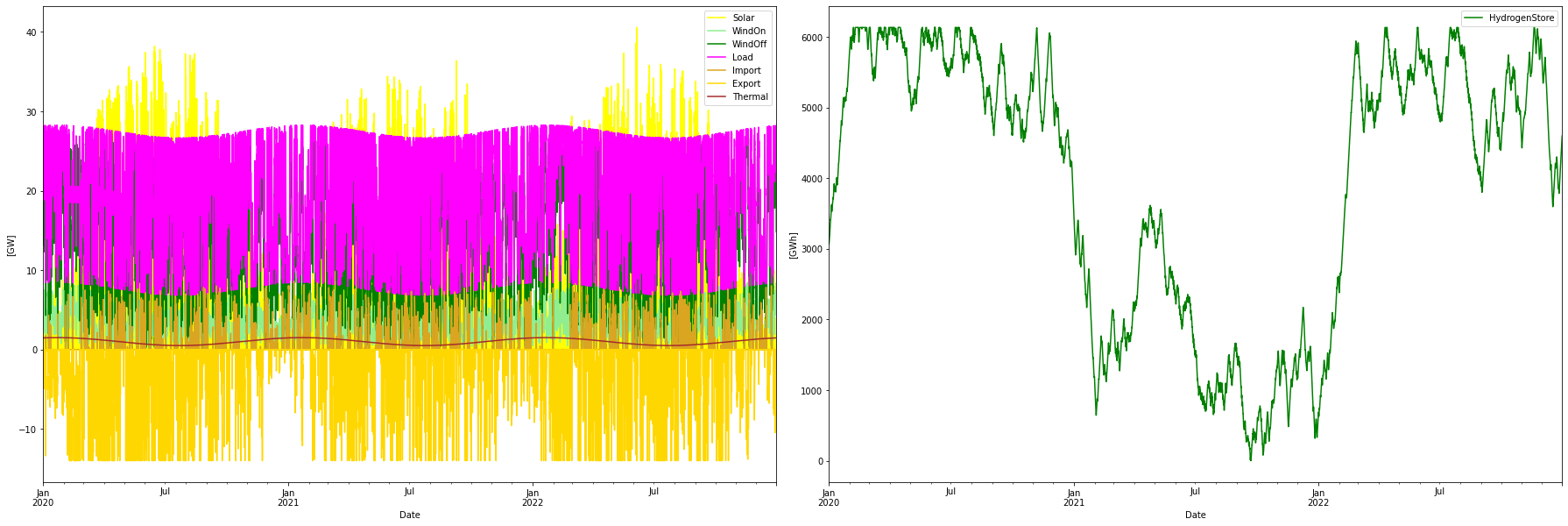
Consumption per year:         165.40 TWh
Consumption H2 per year:       89.69 TWh
Produced WindOn per year:      20.51 TWh
Produced WindOff per year:    105.43 TWh
Produced solar per year:       47.08 TWh
Produced thermal per year:      8.77 TWh
Curtailed per year              2.49 TWh
Deficit per year               -0.00 TWh
Import per year:                5.72 TWh
Export per year:               19.62 TWh
Max overshot:                  25.69 GW
Max shortage:                   0.00 GW

Yearly energy balance
---------------------
Total supply:                 187.51 TWh
Total demand:                 187.51 TWh
Balance:                       -0.00 TWh

Yearly H2 store balance
-----------------------
Total produced:                89.69 TWh
Total delivered:               89.20 TWh
Store change:                   0.49 TWh
Balance:                        0.00 TWh

                  Installed Capacity Unit  TWh/year  CAPEX/GW(h)  OPEX/MW(h)/y   CRF  Tot CAPEX  Tot OPEX  Ann Cost    LCOE
WindOn                        6.503   GW    20.509        1.000        30.000 0.078      6.503     0.195     0.704  34.318
WindOff                      22.708   GW   105.427        2.500        75.000 0.078     56.769     1.703     6.144  58.277
Solar                        31.615   GW    47.081        0.500        15.000 0.078     15.808     0.474     1.711  36.337

Thermal                       2.700   GW     8.768        1.500       468.400 0.066      4.050     1.265     1.534 174.937
H2Store                    6132.000  GWh     0.000        0.001         0.000 0.078      6.132     0.000     0.480     inf
H2Elys                       17.830   GW     0.000        0.500        15.000 0.078      8.915     0.267     0.965     inf
Import                        1.000  N/A     5.721        0.000       856.056 0.060      0.000     0.856     0.856 149.640
Export                        1.000  N/A    19.621        0.000      -428.400 0.060      0.000    -0.428    -0.428 -21.833

Total over-night cost           98.2 GUSD
Total yearly OPEX costs          4.3 GUSD
Annualized cost              11.9647 GUSD
System LCOE                  72.3395 USD/MWh
Scenario 2: RE + Nuclear optimized
In this scenario, nuclear power is added to the mix. It is done by assuming 16 reactors, all having the same power capacity, summing up to a total nuclear power capacity. Each reactor has random on/off-line times (Markov chain), providing a varying total output, here with a capacity factor of 89.9%
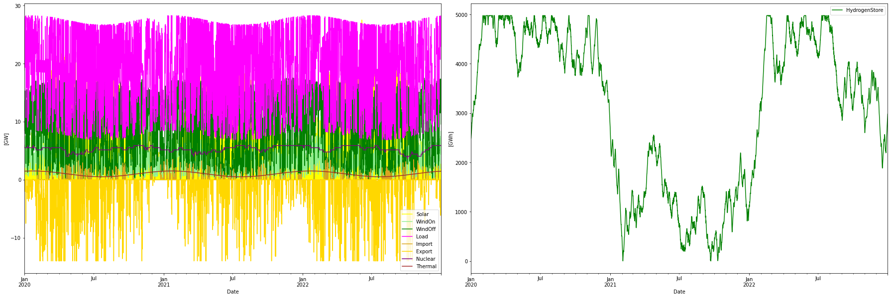
Consumption per year:         165.06 TWh
Consumption H2 per year:       89.36 TWh
Produced WindOn per year:      20.51 TWh
Produced WindOff per year:     68.02 TWh
Produced solar per year:       31.93 TWh
Produced thermal per year:      8.77 TWh
Produced nuclear per year:     46.30 TWh
Nuclear capacity factor:        89.91 %
Curtailed per year              0.41 TWh
Deficit per year               -0.00 TWh
Import per year:                0.64 TWh
Export per year:               10.69 TWh
Max overshot:                  13.85 GW
Max shortage:                   0.00 GW

Yearly energy balance
---------------------
Total supply:                 176.16 TWh
Total demand:                 176.16 TWh
Balance:                       -0.00 TWh

Yearly H2 store balance
-----------------------
Total produced:                89.36 TWh
Total delivered:               89.20 TWh
Store change:                   0.16 TWh
Balance:                        0.00 TWh

                  Installed Capacity Unit  TWh/year  CAPEX/GW(h)  OPEX/MW(h)/y   CRF  Tot CAPEX  Tot OPEX  Ann Cost    LCOE
WindOn                        6.503   GW    20.509        1.000        30.000 0.078      6.503     0.195     0.704  34.318
WindOff                      14.650   GW    68.017        2.500        75.000 0.078     36.625     1.099     3.964  58.277
Solar                        21.438   GW    31.925        0.500        15.000 0.078     10.719     0.322     1.160  36.337
Nuclear                       5.873   GW    46.297        5.000       229.000 0.062     29.365     1.345     3.162  68.296
Thermal                       2.700   GW     8.768        1.500       468.400 0.066      4.050     1.265     1.534 174.937
H2Store                    4977.600  GWh     0.000        0.001         0.000 0.078      4.978     0.000     0.389     inf
H2Elys                       17.830   GW     0.000        0.500        15.000 0.078      8.915     0.267     0.965     inf
Import                        1.000  N/A     0.644        0.000        88.315 0.060      0.000     0.088     0.088 137.104
Export                        1.000  N/A    10.690        0.000      -355.727 0.060      0.000    -0.356    -0.356 -33.277

Total over-night cost          101.2 GUSD
Total yearly OPEX costs          4.2 GUSD
Annualized cost              11.6104 GUSD
System LCOE                  70.3391 USD/MWh
Scenario 3: Manually adjusted RE + Nuclear mix
This scenario builds from Scenario 2 but is manually adjusted to cost the same as Scenario 1. That is roughly 3% over the optimized mix. We can see that this manual adjustment provides a completely different set of characteristics.
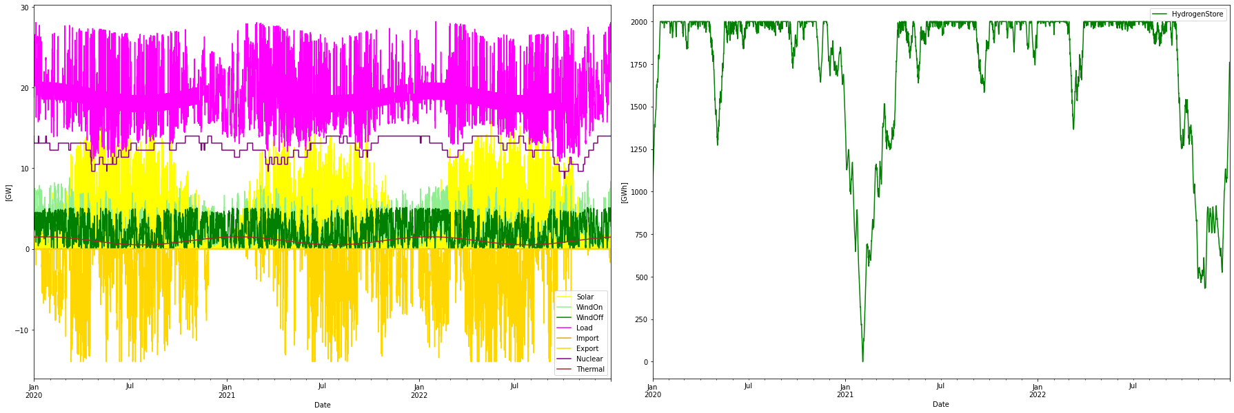
Consumption per year:         165.16 TWh
Consumption H2 per year:       89.46 TWh
Produced WindOn per year:      20.51 TWh
Produced WindOff per year:     20.01 TWh
Produced solar per year:       19.96 TWh
Produced thermal per year:      8.77 TWh
Produced nuclear per year:    110.36 TWh
Nuclear capacity factor:        89.91 %
Curtailed per year              0.06 TWh
Deficit per year               -0.00 TWh
Import per year:                0.00 TWh
Export per year:               14.38 TWh
Max overshot:                   4.08 GW
Max shortage:                   0.00 GW

Yearly energy balance
---------------------
Total supply:                 179.61 TWh
Total demand:                 179.61 TWh
Balance:                        0.00 TWh

Yearly H2 store balance
-----------------------
Total produced:                89.46 TWh
Total delivered:               89.20 TWh
Store change:                   0.27 TWh
Balance:                        0.00 TWh

                  Installed Capacity Unit  TWh/year  CAPEX/GW(h)  OPEX/MW(h)/y   CRF  Tot CAPEX  Tot OPEX  Ann Cost    LCOE
WindOn                        6.503   GW    20.509        1.000        30.000 0.078      6.503     0.195     0.704  34.318
WindOff                       4.310   GW    20.011        2.500        75.000 0.078     10.775     0.323     1.166  58.277
Solar                        13.403   GW    19.959        0.500        15.000 0.078      6.701     0.201     0.725  36.337
Nuclear                      14.000   GW   110.363        5.000       229.000 0.062     70.000     3.206     7.537  68.296
Thermal                       2.700   GW     8.768        1.500       468.400 0.066      4.050     1.265     1.534 174.937
H2Store                    2000.000  GWh     0.000        0.001         0.000 0.078      2.000     0.000     0.156     inf
H2Elys                       17.830   GW     0.000        0.500        15.000 0.078      8.915     0.267     0.965     inf
Import                        1.000  N/A     0.000        0.000         0.000 0.060      0.000     0.000     0.000     NaN
Export                        1.000  N/A    14.382        0.000      -839.097 0.060      0.000    -0.839    -0.839 -58.343

Total over-night cost          108.9 GUSD
Total yearly OPEX costs          4.6 GUSD
Annualized cost              11.9486 GUSD
System LCOE                  72.3437 USD/MWh
Discussion and conclusions
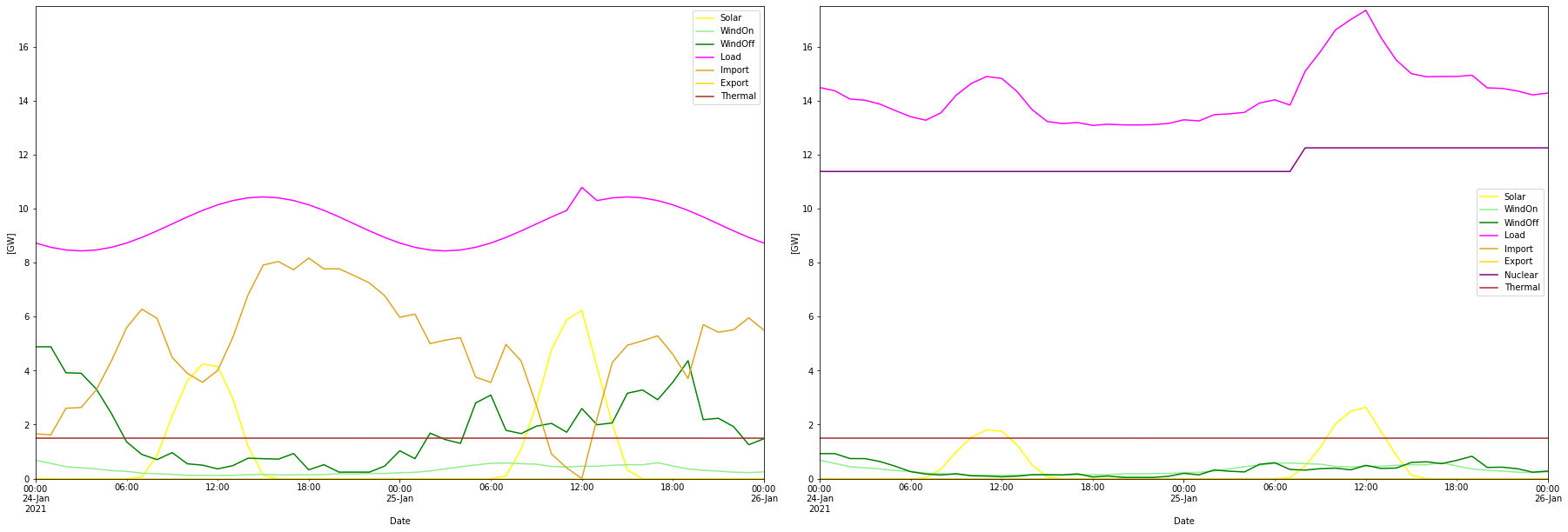
The two cost-optimal scenarios 1 and 2 show similar features. Scenario 2 is somewhat more cost-effective and trims down the need for import and storage size. While not included in the model, Scenario 2 also provides needed system services such as inertia. In Scenario 2 the 5.9 GW total nuclear capacity is split on 16 reactors, giving a power of 370 MW each. This would correspond to large SMRs. Given these could be built we would get an incrementally better system.
But the real improvement is given in Scenario 3 with the same cost as Scenario 1. Here the large dispatch of nuclear power offsets a lot of the variable RE power and provides a much more balanced system. In scenario 3 each reactor gets a nominal power of 875 MW. The Markov chain simulation of the 16 reactors in Scenario 2 gives a power out swing of 2.2 GW between max (that is 5.9 GW) and min (3.7 GW). In Scenario 3 the same Markov chain is used and since the reactors are 14/5.9 times larger, the swing is also this much larger, i.e. 5.2 GW ( or from 14 to 8.8 GW).
The relatively low swing of nuclear power together with the decreased swing of the RE sources in Scenario 3 provides for a much more balanced system. This is manifested in a lower overshot ( 4 vs 27 GW) and lower curtailment (0.06 vs 2,5 TWh) and an eliminated need for import ( 0 vs 5.7 TWh). Also, the storage need decreases substantially, from 6 to 2 TWh worth of hydrogen.
The model does not take transmission and stabilization costs into account, but most probably both these cost types will be smaller in the more balanced Scenario 3 system. If these costs were taken into account, Scenario 3 would probably not just become the most well-balanced system, and best from an energy security point of view (since not import dependent), but also the system with the lowest cost.
Another observation is that cost minimization as a decision tool is rather blunt, since widely different configurations may turn out to cost about the same. Especially if an error margin is taken into account, then it would be hard to say which of the three scenarios has the lowest cost. The value of these models is more that they shed some light on the different characteristics of the solutions.
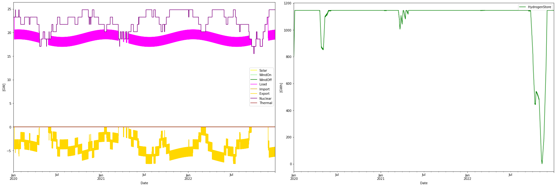
Update: Nuclear only alternative
A question from Oscar L. Martin on LinkedIn prompted me to whip together a simulation of only nuclear + hydrogen storage for hydrogen production flexibility and that was quite interesting!
The optimized mix became 24.8 GW of nuclear power and 1.1 TWh of hydrogen storage. An export of 30 TWh at a capture rate of 70 USD/MWh (and no import) contributed to the low system cost. How the model achieves this capture rate is a little bit fishy, but on the other hand, it is not unreasonable, the capture rate could even be higher since the nuclear power output is correlated to the demand in the winter, given that maintenance is done during the summer.
It was also possible to shave off a couple of unused GWs from the electrolyzer which then became 15.2 GW instead, also contributing to a lower System LCOE which then became (including the contribution from export, same as in the other simulations) became 73.4 USD/MWh, close to the 72.3 USD/MWh for the RE-only alternative. Utilization factor of the electrolyzers becomes somewhat higher, 67% instead of 57%.
Again, overproduction of nuclear power combined with hydrogen production flexibility (note! _not_ hydrogen gas turbine flexibility) is seen to be an interesting prospect.
Consumption per year:         165.02 TWh
Consumption H2 per year:       89.31 TWh
Produced nuclear per year:    195.64 TWh
Nuclear capacity factor:        89.91 %
Curtailed per year              0.00 TWh
Deficit per year               -0.00 TWh
Import per year:                0.00 TWh
Export per year:               30.62 TWh
H2flex per year:                0.76 TWh
H2over per year:               -0.87 TWh
Max overshot:                   0.00 GW
Max shortage:                   0.00 GW

Yearly energy balance
---------------------
Total supply:                 195.64 TWh
Total demand:                 195.64 TWh
Balance:                        0.00 TWh

Yearly H2 store balance
-----------------------
Total produced:                89.31 TWh
Total delivered:               89.20 TWh
Store change:                   0.11 TWh
Balance:                        0.00 TWh

                  Installed Capacity Unit  TWh/year  CAPEX/GW(h)  OPEX/MW(h)/y   CRF  Tot CAPEX  Tot OPEX  Ann Cost    LCOE
Nuclear                      24.818   GW   195.640        5.000       229.000 0.062    124.089     5.683    13.361  68.296
H2Store                    1145.700  GWh     0.000        0.001         0.000 0.078      1.146     0.000     0.090     inf
H2Elys                       15.200   GW     0.000        0.500        15.000 0.078      7.600     0.228     0.823     inf
Import                        1.000  N/A     0.000        0.000         0.000 0.060      0.000     0.000     0.000     NaN
Export                        1.000  N/A    30.621        0.000     -2167.944 0.060      0.000    -2.168    -2.168 -70.799

Total over-night cost          132.8 GUSD
Total yearly OPEX costs          3.7 GUSD
Annualized cost              12.1056 GUSD
System LCOE                  73.3596 USD/MWh
Hydrogen storage in Denmark
A last aspect is the hydrogen storage possibilities in Denmark. Luckily they have the right geological conditions for this. According to Gas Storage Denmark they can store about 10.8 TWh of NG energy. I have tried to convert that to the corresponding number for hydrogen and get it to a factor of about 4-5 less hydrogen energy in the same storage. (Would be glad if someone knowledgeable could confirm and correct this factor). This would mean that 2.4 TWh of hydrogen LHV energy could be stored, corresponding to 3.6 TWh of electricity to produce this amount of H2, which is the unit used for storage in this blog post.
3.6 TWh is too little for Scenarios 1 and 2 that demanded 6 and 5 TWh respectively. But for Scenario 3 (more nuclear) and for the nuclear-only alternative the storage would suffice, because these need 2 and 1 TWh respectively.