
Bengt J. Olsson
Twitter: @bengtxyz
LinkedIn: beos
Oliver Ruhnau and Staffan Qvist (“RQ”) presents a very illuminating analysis of Germany’s storage need for a fossil free 540 TWh consumption scenario here (and here in a short Twitter thread). Basically, their power system is fueled with 700 TWh of renewable energy for a consumption of 540 TWh. The difference is accounted for by 90 TWh curtailed energy and the rest are round-trip losses in the energy storages.
The real achievement in the paper is to conclude that a hydrogen store of 54.8 TWh (H2 LHV) is needed to account for the lowest wind conditions during a 37-year period.
Their model produces a cost optimal system given input CAPEX and OPEX for each (investable) system component, given a set of boundary conditions. No import or export is allowed, and the model supposes a “copper plate” transmission network, that is transmission is not included, just to supposed to be in place without limitations.
The RQ paper is very complete and thorough and there isn’t much to add to it. But anyway, in this blog post I will compare the output of my SWENS (Solar, Wind, Eco, Nuclear, Storage) model with the RQ model, using as similar assumptions as possible. This will provide a sort of “benchmark” for the SWENS model, or at least a reality check.
And in conclusion, the results from the SWENS model are both qualitatively and quantitatively in good agreement with the RQ paper, which is incouraging and will lead to further exploration with this model.
Power/Energy balance
In the SWENS simulation similar cost parameters as in the RQ paper are used. There are still some differences due to how Eco power (biomass, hydro run of river, etc) and pumped hydro (PHS) is handled, but the major parts, solar, wind and hydrogen storage are using the same cost parameters. The SWENS simulation runs with scaled wind and solar data from ENTSO-E for the years 2020-2022, that is over three years, while RQ uses time series data for a period 1982-2016. An optimization is performed to minimize the yearly annualized cost, with the (only) condition applied is that no deficit shall occur. Output from the simulation is
Consumption per year:         540.11 TWh
Produced windOn per year:     210.09 TWh
Produced windOff per year:    313.11 TWh
Produced solar per year:      100.30 TWh
Produced eco+bio per year:     70.14 TWh
Curtailed per year             72.81 TWh
Deficit per year                0.00 TWh
Battery charge per year        -0.76 TWh
Battery discharge per year      0.68 TWh
PH charge per year            -28.49 TWh
PH discharge per year          22.79 TWh
Hydrogen charge per year     -123.64 TWh
Hydrogen discharge per year    48.67 TWh
Import per year:                0.00 TWh
Export per year:                0.00 TWh
Max overshot:                 112.49 GW
Max shortage:                   0.00 GW

               Installed Capacity Unit  TWh/year   Tot CAPEX  Tot OPEX  Ann Cost
WindOn                   109.013   GW   210.090       98.112     1.417     9.092
WindOff                   83.124   GW   313.112      149.623     2.161    13.866
Solar                    104.088   GW   100.300       46.840     1.041     4.705
EcoBio                    16.000   GW    70.144        0.000     0.000     0.000
H2Store*               82200.000  GWh     0.000      123.300     0.000     9.645
H2Elys                    54.500   GW     0.000       24.525     0.490     2.409
H2CCGT                    66.200   GW    48.672       49.650     0.993     4.877
PHStore                    8.850   GW    22.789        0.000     0.000     0.000
BatteryStore               4.700  GWh     0.683        0.667     0.000     0.069

Total over-night cost            493 GEUR
Total yearly OPEX costs            6 GEUR
System LCOE                    0.083 EUR/kWh

*) H2 store value adjusted from optimied value of 24.700 GWh for time series data for 2020-2022, to the worst case value from the RQ paper in order to correctly compare the total cost.
As we can see we have wind and solar power generation values similar to the RQ paper. The 70 TWh EcoBio is an assumed generation of mostly biomass and hydro run of river power, but also other smaller sources that are assumed to produce the same amounts as today, that is about 8 GW constant power. (See for instance this chart).
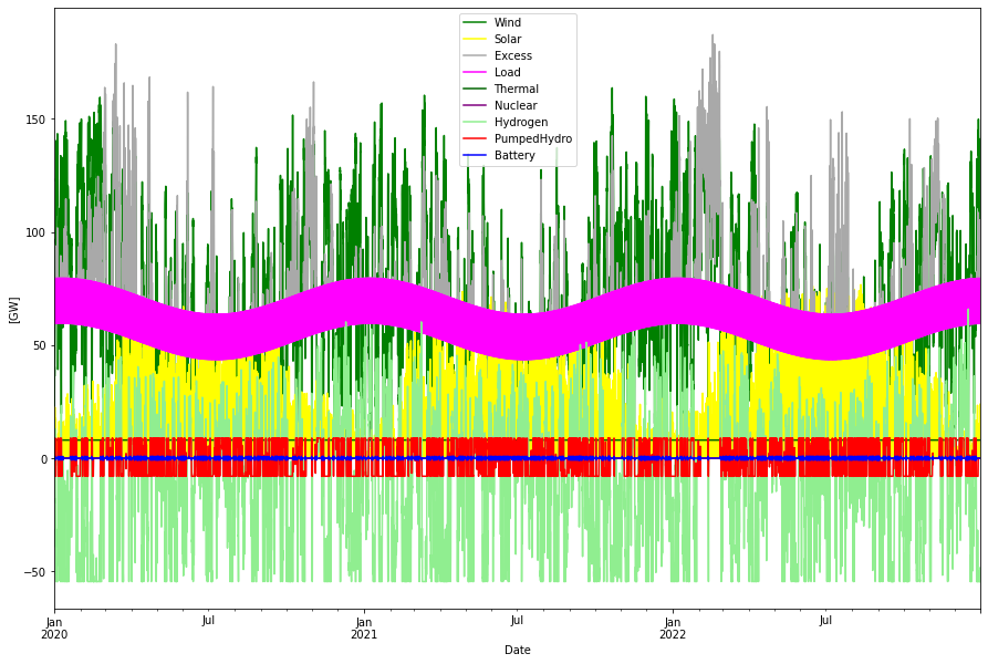
Production and consumption is balanced using the three storage options Battery, Pumped Hydro (PHS), and Hydrogen. The dispatch order is Battery -> PHS -> Hydrogen (both for charge and dis-charge). The balance can be written as:
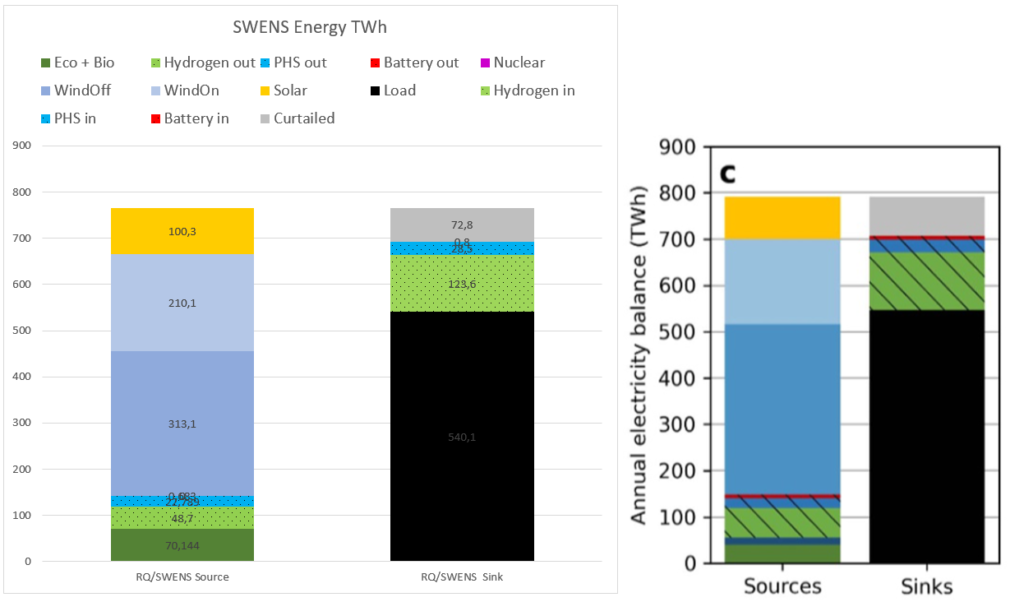
Produced: 210.1 + 313.1 + 100.3 + 70.1 + 48.7 + 22.8 + 0.7 = 765.8 TWh
Consumed: 540.1 + 72.8 + 123.6 + 28.5 + 0.8                = 765.8 TWh
Here is a comparison of the energies obtained in this simulation vs the similar simulation in the RQ paper
They show a good agreement in terms of balance between wind, solar, hydrogen and PHS power. The total wind energy is somewhat lower with 523 TWh vs 550 in the RQ paper. This is partly compensated by more solar (100 vs 90 TWh), more energy from the fixed Eco part (biomass and hydro ror plus other) and lower curtailment.
The most striking difference is that battery storage (and power) is very low in the SWENS simulation. In the RQ model the battery storage is 60 GWh, but here it is almost wiped out to only 4.7 GWh.
In the graph above we can see the inter-play between the different power sources, storages and consumption.
It was interesting to see that in optimization the ratio between onshore and offshore wind varied quite much with little cost difference. This is probably explained by the cost parameter setting in the RQ model. Off shore wind power is assigned precisely double the CAPEX and OPEX cost of on shore wind power, at the same time the capacity factor for off shore wind is almost exactly twice that of on shore wind. This makes the cost per produced kWh almost the same. If then the properties of the produced power is similar it does not really matter if it is on or off shore wind that produces the energy. Since off shore wind is still favored it probably exhibits a more even production over the year.
Storage aspects
Storages are modelled as objects with attributes power in and out capacities, a size and a round-trip efficiency. An update fill level methode provides the current fill level of each storage.
Three types of storages: batteries, PHS and hydrogen are considered. Battery storage is first activated but since it only keeps 4.7 GWh it quickly runs empty. PHS has a higher storage capacity of 1.28 TWh and last a little bit longer. But the largest part of the balancing is done with the hydrogen store that handles the seasonal (and longer) balancing. This simulation uses the same storage properties as in the RQ paper, except for hydrogen storage where a 40% rount-trip efficiency for
power->hydrogen->power is used, instead of the more optimistic 50% in the RQ model.
The fill levels of all three stores are depicted below.
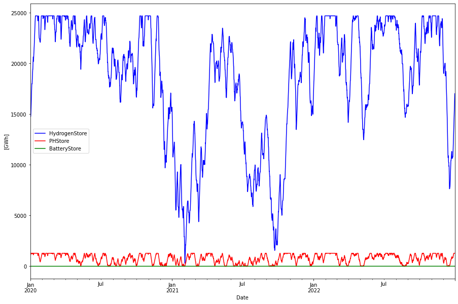
Note that all stores are measured by the energy used to fill the store. This gives a consistent measure that is independent of the losses of the stores. By contrast in the RQ paper the hydrogen store is measured in H2 LHV calorific energy units, 33.3 kWh/kg.
To work with simple numbers, the following energy relations is used here:
Energy consumed to produce hydrogen:   50 kWh/kg
Hydrogen LHV calorific energy units:   33 kWh/kg
Energy generated from CCGT combustion: 20 kWh/kg
This gives a round-trip efficiency power->H2->power of 20/50 = 40%. It also means that the RQ maximum hydrogen store of 54.8 TWh (LHV) must be multiplied by 50/33.3 to get the corresponding input energy measure, which becomes 82.2 TWh.
82.2 TWh is a much too large store for the period 2020-2022 as can be seen above. Actually around 25 TWh (or 16.7 TWh LLV) would have been enough, but since hydrogen is the last backup resort in this model, the store should be large enough to handle the worst case.
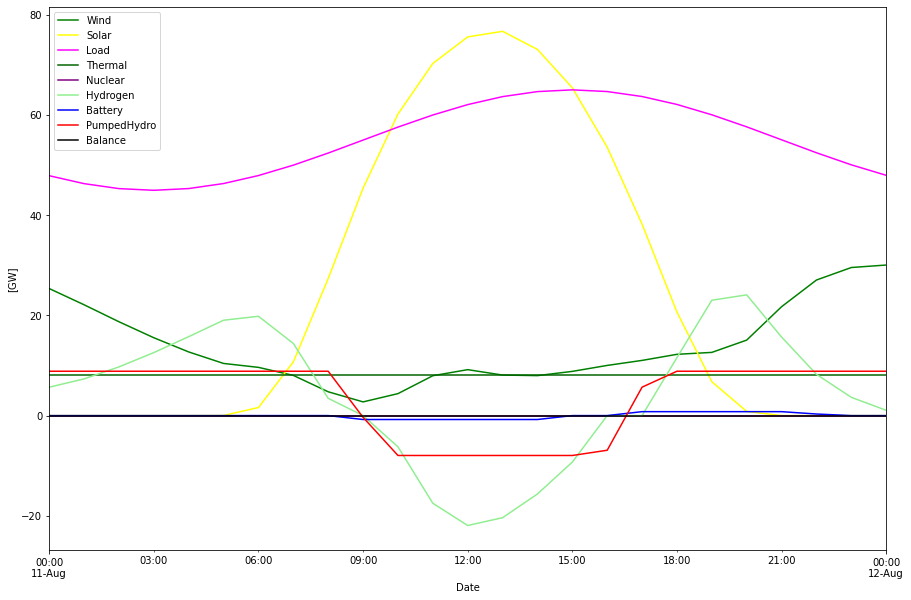
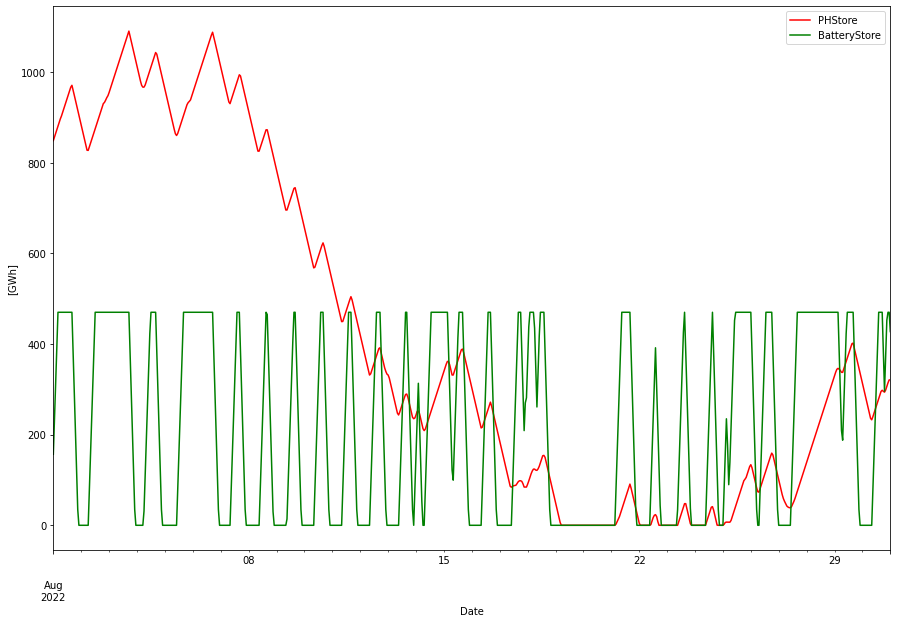
Batteries and PHS contributes much less, but with higher frequency as expected. Below is the fill levels for these expanded for August 2022. Batteries has a more or less daily charge/dis-charge pattern and PHS works on longer time scale.
Cost aspects
LCOE for the total system is estimated to 87 EUR/ MWh. This includes the “non-investible” generators Eco/PHS (which btw are very difficult to estimate costs for). If removing these the RQ comparable value is 83 EUR / MWh, in close agreement with the 80 EUR / MWh that RQ suggests. Also the same split between RE costs (51 EUR / MWh) and storage (31 EUR MWh) is obtained. The difference may be accounted mainly to two factors: Using a slightly higher fixed amount (“Eco”) in this simulation would actually lower the system cost for the SWENS model, since the RE part becomes somewhat smaller. On the other hand, using a 50% round-trip efficiency of the hydrogen storage system will lower the total system cost in the RQ model. Enough to say that they are in the same ballpark of total cost.
Actuall costs used (CAPEX: GEUR, OPEX: MEUR):
		CAPEX/GW(h)	OPEX/MW(h)
WindOn		0.9		13
WindOff		1.8		26
Solar		0.45		10
Nuclear		-		-
(EcoBio		4.771		146.3)
H2Store		0.002		0
H2Elys		0.45		9
H2CCGT		0.75		15
(PHStore	2.738		20)
BatteryStore1	0.142		0
EV flexibility
What about electrical vehicles (EV) with their batteries? It is forecasted that EVs in Germany may have 50 -100 TWh of battery storage capacity from EVs in the future. Won’t they contribute to the energy storage? Yes but here these are accounted for on the consumption side.
In this coarse model, consumption is modeled as long sinusoidal for season variation and a short sinusoidal for daily variation. (Over the year the sum is 540 TWh). This is of course not a correct pattern but it is “good enough” to model longer times average behavior. It probably somewhat underestimates sudden power peaks and shortages though.
The effect of large scale EV charging is likely that the “daily sinusoidal” gets a lower amplitude since EV owners likely will charge their cars over the night and hence move consumption from the day to the night. At least in the darker seasons, in the summer also abundant solar power may be absorbed for charging. This is however not modeled here.
Hydrogen production/flexibility
The excess/curtailed energy can of course be used for export and/or hydrogen production for industrial use. If used for hydrogen production, in principle 63 TWh (or 42 TWh LLV) could be produced if adding 113 GW of electolyzer capacity on top of the 54.5 GW that is already used for the energy store production. This would give a mere 6.4% utilization of the extra electrolyzer capacity, vs 28% capacity factor for the energy storage electrolyzers.
Given the low capacity factor obtained for industrial hydrogen production, it will be very expensive. A more optimal power system for the production of industrial hydrogen takes this production into account as a flexible load and is designed after these needs. (See for example this blog post for more on hydrogen production and storage).
Summary
Even though the models simulate different time series data, the results are in good agreement. This encourages me to further exploit the SWENS model. In a follow-up blog post I will use the SWENS model but updated with both new cost estimates and capacity factors, and also include nuclear power into the mix. Stay tuned… and here it is!
Footnotes
- The battery storage is somewhat simplified in this model. Instead of having two independent optimization variables for the inverter size and battery pack respectively, this model locks the inverter size to the storage size by stipulating that 6 hours battery stores are used (as concluded in the RQ paper). That is the inverter capacity in GW is equal to the storage capacity in GWh dividev by 6h. ↩︎