
Bengt J. Olsson
X: @bengtxyz
LinkedIn: beos
Contents:
Model and Objectives
Scenario 1: Wind + Solar + Hydrogen
Scenario 2: Nuclear + Hydrogen
Observations and Key findings
Fully optimized system
Appendix 1: Cost Assumptions
Appendix 2: Overprovisioning vs Storage?
Appendix 3: Seasonal load variation
Sometimes it’s useful to take a step back for a broader perspective. Today’s energy system models are often highly complex and rely on a multitude of assumptions—some uncertain. While such models provide important insights, a simplified framework can be valuable for identifying major trends and structural characteristics.
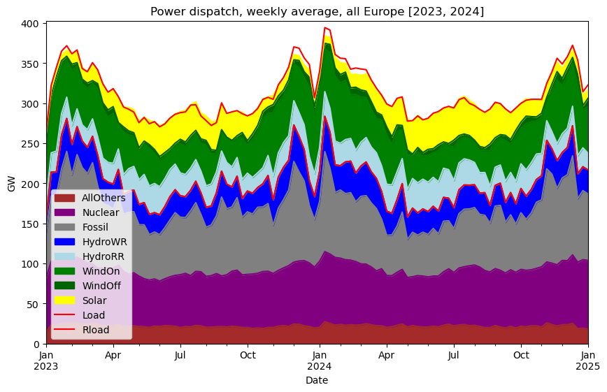
This post presents such a simplified model to explore how a fossil-free European power system might be built by 2050. The model is based on aggregated EnergyCharts (EC) data for 2023–2024 and treats Europe as one unified country with no internal transmission constraints—a classic “copper-plate” assumption. All generation and consumption is summed to roughly 2750 TWh/year. Import and export flexibility, that typically is subject to large uncertainties, becomes void in this model, as Europe is treated as one closed system without borders.
Model and Objectives
Two fossil-free scenarios for 2050 are analyzed:
• Scenario 1 (WS): Expansion of wind and solar power, with nuclear and other power sources held constant at 2023-2024 levels according to EC
• Scenario 2 (NUC): Expansion of nuclear power, while wind, solar, and other sources are held constant instead
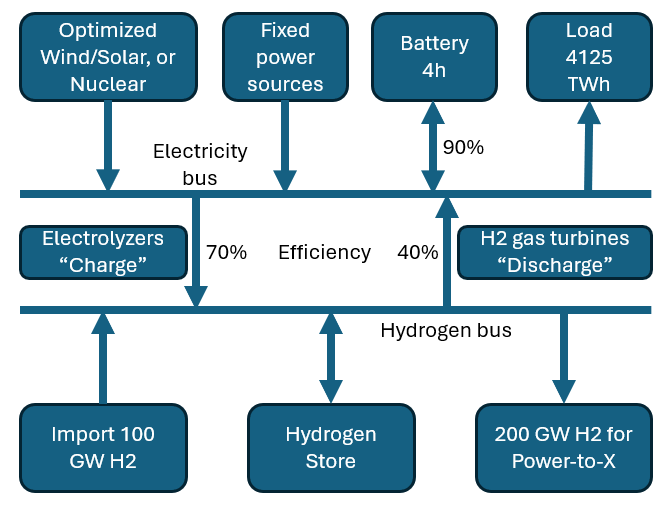
Both scenarios include hydrogen production and storage, as well as battery support. All fossil-based power generation is, of course, removed. The future electricity demand is assumed to be approximately 4125 TWh/year (50% above today’s level), plus an additional 1750 TWh/year of hydrogen for the Power-to-X sector. Half of this hydrogen is assumed to be imported, so the model must deliver 875 TWh or 100 GW of continuous hydrogen output to industry. The linear scaling of load is motivated by the assumption that many new demand sources—such as electrified transport, data centers, and industrial processes—will add relatively constant load throughout the year. But, in contrast, the shift from gas boilers to electric heat pumps will amplify the seasonal variations in electricity demand. This validity of this assumption is further elaborated in Appendix 3 below.
Electrolyzer efficiency (electricity → H₂) is set at 70%, and hydrogen turbine efficiency (H₂ → electricity) at 40%. Batteries are assumed to have a 4-hour capacity and 90% round-trip efficiency. The model is optimized using PyPSA to find the lowest total system cost under these conditions. The assumed costs for all components are listed in Appendix 1 below.
The rationale for keeping all other power sources—such as hydro, biomass, and others—at their nominal 2023–2024 hourly values is that, since they are not expanded in this model, they would likely operate at similar levels as today. This is consistent with the assumption that the load curve retains a similar shape in the future.
Scenario 1: Wind and Solar Expansion (WS)
In this scenario, a constraint is imposed such that onshore wind may be expanded to at most three times today’s installed capacity, and solar power to a maximum of ten times. These limits mean that the remaining demand must be met by offshore wind, despite its higher cost.
To estimate capacity factors, we use EnergyCharts (EC) data for installed capacity and actual generation in 2024. The results for all of Europe are:
• Onshore wind: 23% (EC) → 30.5% in 2050 (higher performance from newer turbines)
• Offshore wind: 43% (EC) → 39.5% in 2050 (lower correlation due to more distributed geography)
• Solar PV: 11% (EC) → 11% in 2050 (assumed unchanged)
For both onshore wind and solar, the maximum instantaneous output in 2024 was around 60% of installed capacity. This suggests low spatial and temporal correlation across Europe — production is spread out geographically and temporally. In the model, the effective capacity factor for onshore wind is adjusted upward to reflect improved technology, while the offshore wind factor is adjusted slightly downward to account for more dispersed and less correlated resources. The observed solar capacity factor remains unchanged in the projection.
Nuclear power, at the present level according to EC data for 2023-2024, is included in the “Fixed” generation capacity, together with all other present generation, except wind and solar power. In this scenario it is thus only wind and solar power that are expanded to meet the higher future load.
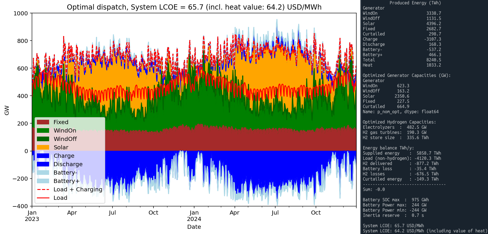
Results for Scenario 1:
Scenario 2: Nuclear Expansion (NUC)
In the nuclear expansion scenario, the model introduces a slow form of load-following: nuclear power is allowed to ramp up from zero to full capacity over one week, and the same ramp-down time applies. In practice, however, the actual variation turns out to be significantly smaller than this theoretical maximum — for reasons discussed later. In the simulation, nuclear output varies by no more than about 12%.
An additional constraint in the model is that nuclear generation is limited to a maximum of 80% of installed capacity. This is a conservative assumption and does not reflect actual operating conditions — in winter, nuclear plants in Europe often operate at over 95% of capacity. However, this cap offers a simple way to account for reduced availability due to maintenance, outages, and inspections.
To be clear, wind and solar power at the present level, according to EC data for 2023-2024, is included in the “Fixed” generation capacity, together with all other present generation, except nuclear. In this scenario it is thus only nuclear power that is expanded to meet the higher future load.
The resulting capacity factor for nuclear power in this scenario is 79.7%.
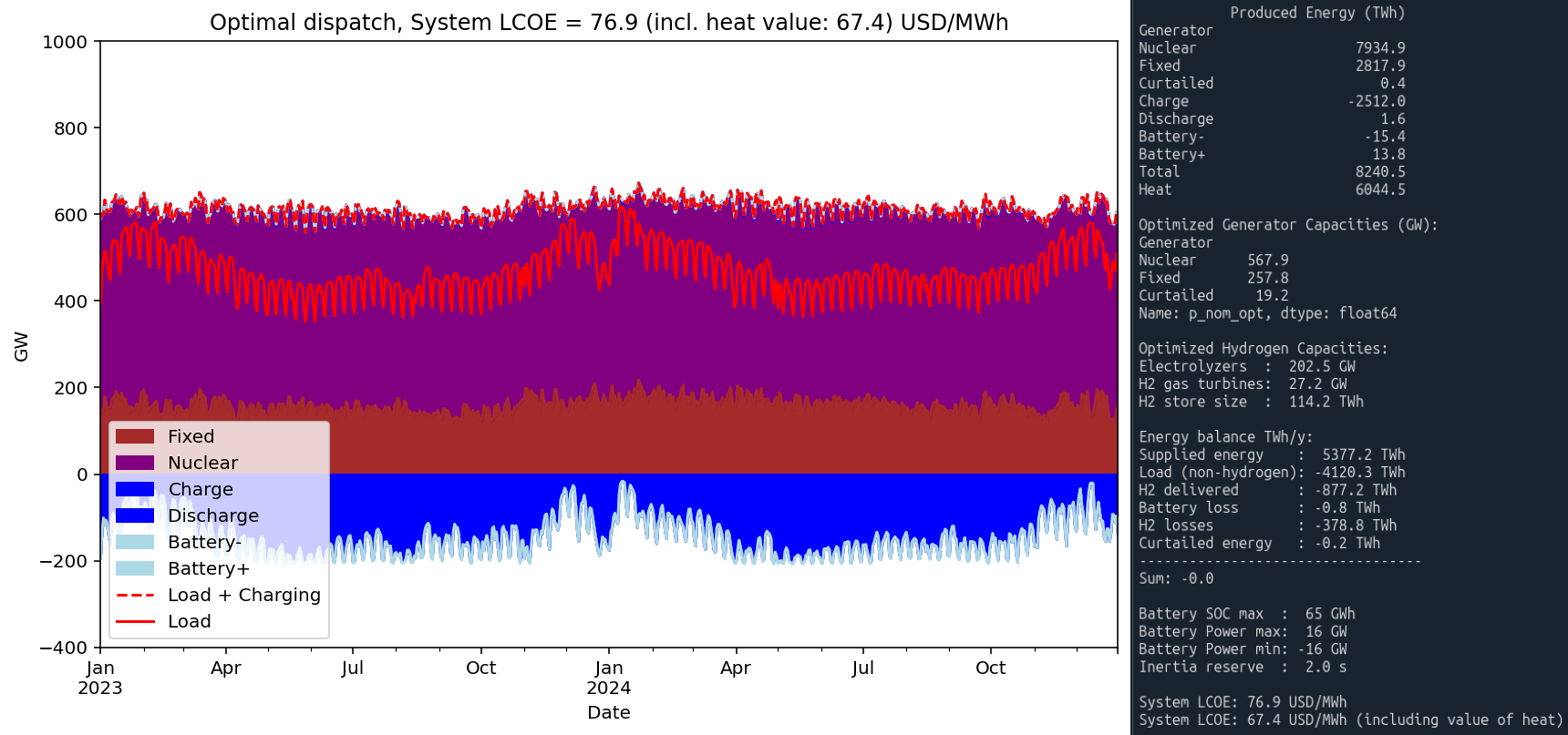
Results for Scenario 2:
Observations and Key Findings
Generation Mix
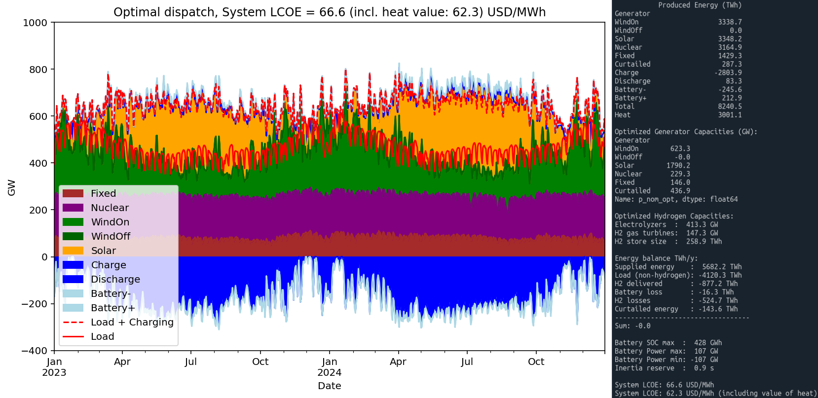
In Scenario 1 — wind and solar (WS) — the model builds out all permitted onshore wind capacity, which corresponds to a threefold increase over today’s installed base, reaching around 620 GW. At the same time, the assumed capacity factor increases by 33%, meaning more energy per unit capacity. Offshore wind is expanded to 163 GW, and solar power is scaled up to the model-imposed limit of 2.35 TW, or ten times the current level.
This enormous amount of solar capacity results in sharp production spikes, with peak output reaching 1,715 GW. Such high peaks pose a serious challenge for transmission infrastructure, both in terms of capacity and system stability.
In contrast, the nuclear scenario (NUC) yields a much more stable electricity output. Peak generation reaches 712 GW — over 1 TW less than in the WS scenario. Nuclear capacity is expanded by a factor of six compared to today’s level, although this figure is somewhat overstated due to the 80% utilization constraint in the model.
Batteries
Batteries play a critical role in both scenarios. In the WS case, 240 GW / 1 TWh of battery capacity is deployed — a substantial volume, alson in 2050. The batteries help shave solar production peaks, easing the load on the transmission grid. This enables a lower capacity of electrolyzers to be installed, while also improving their utilization. On the demand side, batteries help reduce the need for hydrogen gas turbines. Altogether, this significantly lowers the LCOE in the WS scenario. The peak-shaving functionality also improves grid operability.
Still, the overall production dynamics in WS remain highly volatile, with rapid changes and steep peaks as mentioned above.
In the NUC case, battery deployment is much more modest — 16 GW / 65 GWh — but the need for flexibility is also much lower due to the steadier output. A particularly noteworthy observation is that all gas turbines in the model could theoretically be replaced with batteries at relatively low cost. In that case, all hydrogen production could be dedicated to the Power-to-X sector.
In addition to bulk balancing, batteries also offer important ancillary services such as frequency control, congestion relief, and local balancing — though these functions fall outside the scope of this model.
Flexibility
At the all-European level, only hydrogen offers sufficient flexibility to balance generation and growing demand in 2050. Other sources such as batteries, pumped hydro, demand-side management (DSM), and hydro reservoirs play important local roles but are comparatively minor on a system-wide scale — particularly in the WS scenario. (For reference, see this post about balancing contributions to the present pan-European power system).
In the WS case, flexibility requires:
• Production flexibility via high-capacity electrolyzers (~500 GW)
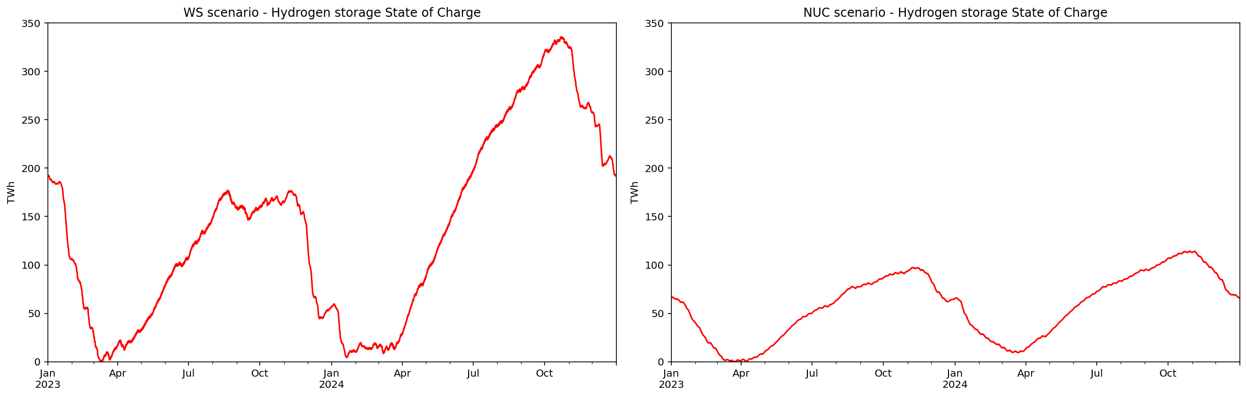
• Storage capacity (~300 TWh)
• Hydrogen turbines (~200 GW) to reconvert hydrogen into electricity when needed
Despite this large infrastructure, approximately 3% of total electricity production is curtailed — i.e., cannot be utilized.
In the NUC scenario, the flexibility requirement is much smaller. The system is almost entirely balanced through variations in hydrogen production over time. Gas turbines play a negligible role. As shown in the output graphs, it is the hydrogen production rate that varies most in this scenario.
Although the model allows for slow load-following by nuclear power, this ability is barely utilized in practice. Nuclear output remains nearly constant throughout the year. The reason is economic: it is cheaper to adjust hydrogen production than to lower nuclear capacity factors. When there is excess power, or lower load, hydrogen production is ramped up rather than throttling nuclear output. This increases storage needs slightly, but the cost is much lower than leaving nuclear reactors idle.
This creates a highly efficient synergy between nuclear and hydrogen: nuclear provides stable baseload power, while hydrogen production offers the system’s flexibility*. The total balancing infrastructure required in the NUC scenario is far smaller than in WS — about 200 GW of electrolyzers, 100 TWh of storage, and 27 GW of gas turbines (which, as noted, could feasibly be replaced by batteries).
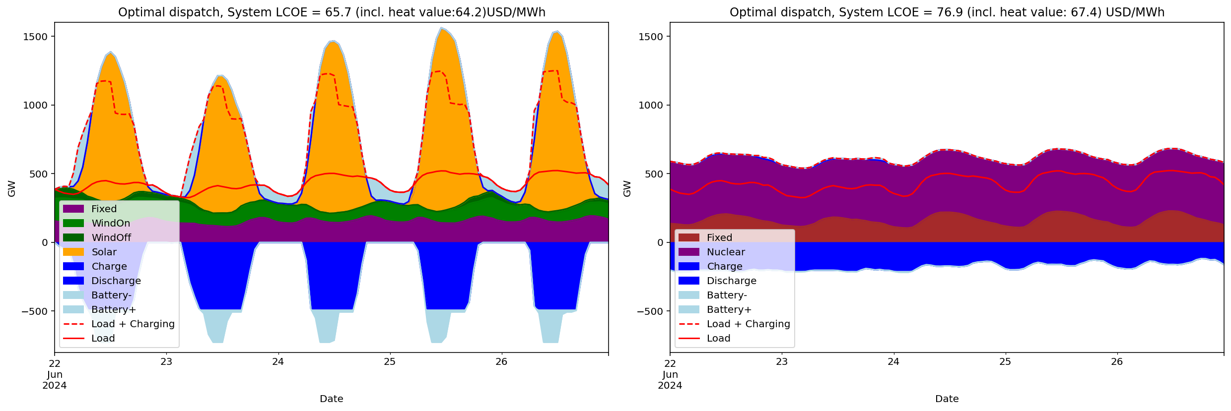
The figure below illustrates how both systems perform during a four-day Dunkelflaute period in December 2024 — a scenario designed to test maximum flexibility needs.
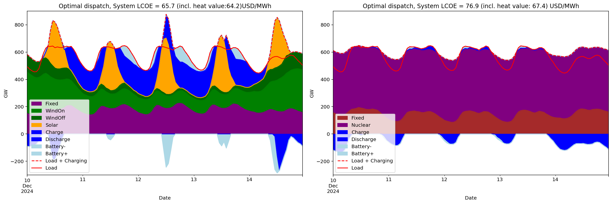
*) The symbiosis between nuclear power and hydrogen storage in the NUC scenario closely resembles the historical interplay between nuclear and hydro reservoir power in Sweden during the 1980s and 1990s. Back then, steady baseload power from nuclear plants in southern Sweden was complemented by the flexible dispatch of hydro power from northern reservoirs. In the NUC scenario, flexible hydrogen production effectively takes on the role that hydro played in balancing the Swedish power system.
System Characteristics
This model does not really account for technical system attributes such as rotational inertia or the costs of balancing forecast deviations and rapid fluctuations in supply and demand. However, the two scenarios differ significantly in how such challenges would likely be managed in practice.
Nuclear power inherently provides synchronous inertia through rotating machinery, which supports frequency stability. The inertial reserve* in the NUC scenario is estimated to about 2 seconds, while in the WS scenario the same estimate is 0.7 seconds. Thus, in the WS scenario, rotaional inertia must instead be achieved via synthetic inertia — for example, through batteries and advanced power electronics — which is feasible but requires more sophisticated control systems.
Overall, the NUC scenario results in a more stable and gradually varying system, while the WS scenario exhibits more pronounced variability in power flows. This increases demands on the transmission grid and on ancillary services. Both approaches are technically viable but differ in their operational characteristics and system requirements.
*) The inertia reserve is here defined as the (estimated) available system inertia (GWs) divided by average system power consumption (GW)
Cost and System LCOE
The model minimizes total system cost under defined technical and economic constraints. However, the resulting cost — expressed here as System LCOE — is highly sensitive to input assumptions, such as technology costs and performance parameters. For this reason, the results should be interpreted with very much caution.
In this case, the WS scenario yields a slightly lower system cost than NUC, but it’s worth emphasizing that higher grid and system costs associated with WS were not included. With different assumptions — for example, on capacity factors, cost trajectories, or component lifetimes — the ranking between scenarios could reverse entirely.
Thus, System LCOE should not be interpreted as an absolute cost comparison for investment decisions, but rather as a tool for exploring how changes within a scenario affect total system economics.
For instance, replacing all gas turbines in the NUC scenario with batteries increases the System LCOE by about 1%, or approximately 1 USD/MWh (1 öre/kWh).
value of heat
Heat is a by-product of nuclear power generation, hydrogen production via electrolysis, and hydrogen combustion in gas turbines. In a future power system, this heat should be utilized—for example, for district heating or industrial process heat—which gives it a tangible value.
In the model, an alternative LCOE is calculated where the value of recovered heat is subtracted from the annualized cost, thereby reflecting the cost of electricity alone. A conservative assumption is applied to nuclear power: only one-third of the generated heat is credited in order to avoid interference with electricity production. For electrolyzers and gas turbines, however, the full amount of excess heat is considered recoverable.
Assuming an electricity-to-heat value ratio of 4:1, the adjusted LCOE values become:
- LCOE(WS, with heat value): 64.2 USD/MWh (down from 65.7)
- LCOE(NUC, with heat value): 67.4 USD/MWh (down from 76.9)
Fully Optimized System
Finally, a scenario is tested in which wind, solar, and nuclear capacities are all treated as free variables in the optimization. As expected, the result is a hybrid solution combining features of both extreme scenarios.*
Key Findings in the Fully Optimized Scenario
The most striking outcome in this scenario is that the mix of onshore wind, solar, and nuclear effectively eliminates the need for offshore wind. Onshore wind is built out to the model’s upper limit, while solar lands at roughly 8× today’s installed capacity — a level that aligns closely with several professional projections for 2050.
Overall, the resulting system resembles the WS scenario, but with some differences:
- Includes twice today’s nuclear capacity
- A reduced hydrogen infrastructure
- Roughly half the battery storage capacity
It should be stressed, however, that these outcomes are highly sensitive to the underlying cost assumptions. Different investment priorities or cost estimates could lead to different conclusions.
Still, the broader takeaway remains robust:
A diversified mix of technologies consistently outperforms single-path strategies.
*) The optimal LCOE becomes higher than in the WS case which seems contradictory when the only change is that a another optimization variable is added. The reason is that there is another change as well. The “Fixed” power sources, corresponding to legacy power sources with an assigned cost of 50 USD/MWh, here without either of nuclear and wind/solar, constitutes a smaller part of the power mix in this case, and hence the average price becomes higher.
Appendix 1: Cost Assumptions
Capex
| Technology | CAPEX |
|---|---|
| Onshore Wind | 1.2 MUSD/MW |
| Offshore Wind | 3.0 MUSD/MW |
| Solar PV | 0.3 MUSD/MW |
| Nuclear | 6.0 MUSD/MW |
| Gas Turbine (H₂) | 1.0 MUSD/MW |
| Electrolyzer | 0.5 MUSD/MW |
| Hydrogen Storage | 1000 USD/MWh |
| Battery (4h) | 0.2 MUSD/MWh |
OPEX
| Technology | CAPEX Lifetime (years) | FOM (% of CAPEX) | Discount rate |
|---|---|---|---|
| Onshore Wind | 25 | 2% | 6% |
| Offshore Wind | 25 | 2% | 6% |
| Solar PV | 25 | 2% | 6% |
| Nuclear | 60 | 2% (+ VOM/Fuel 10 USD/MWh) | 6% |
| Gas Turbine (H₂) | 25 | 2% | 6% |
| Electrolyzer | 25 | 2% | 6% |
| Hydrogen Storage | 40 | 2% | 6% |
| Battery (4h) | 15 | 2% | 6% |
cost for other power
“Fixed” or legacy power dispatch (with values retained from from EnergyChart’s data) is given a cost of 50 USD/MWh.
Appendix 2: Overprovisioning vs Storage?
Both scenarios rely heavily on hydrogen storage to provide system flexibility. But how dependent are they on this storage? To explore this, a simulation was run where the only change was to fix the hydrogen storage capacity to 1 TWh—instead of letting it be optimized by the model. The same electricity and hydrogen demand profiles were applied as before.
A storage capacity of 1 TWh roughly corresponds to what could be stored in the pipeline network itself—so-called “line-pack” storage. This assumes a hypothetical European hydrogen transmission network consisting of 10,000 km of pipelines, each 1 meter in diameter, with operating pressures varying between 50 and 100 bar.
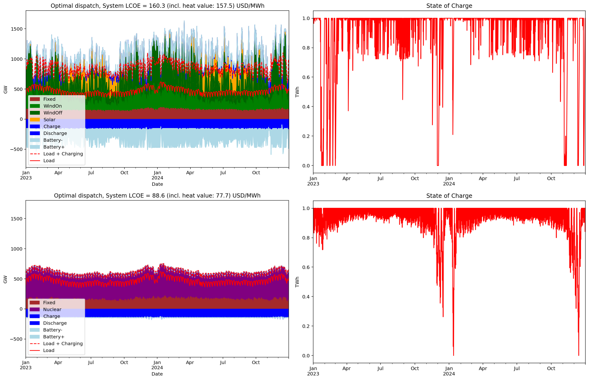
In the WS scenario, a substantial amount of offshore wind power is added—since both onshore wind and solar are already built to their maximum limits—alongside an enormous 13.5 TWh of battery storage. As a result, maximum power dispatch reaches a staggering 2.3 TW. System costs soar to approximately 160 USD/MWh, an increase with 144%.
In contrast, the NUC scenario sees nuclear capacity increase to 726 GW (up from 568 GW), while maintaining a much steadier dispatch profile, now peaking at around 800 GW. System costs increases only 15%, system LCOE becomes nearly half compared to the WS case, and batteries are entirely excluded from the solution.
This illustrates an important point: with fully dispatchable power sources, it is theoretically possible to eliminate the need for flexible energy storage by simply sizing generation to cover peak demand and curtailing output during lower load periods. While not cost-optimal, this potential becomes visible when storage flexibility is removed from the system—as seen in the diverging results between the two scenarios.
Appendix 3: Estimating seasonal load variation
Seasonal variation in electricity demand plays a crucial role in determining the results of this simulation, most notably, in the need for balancing and the sizing of hydrogen storage. In fact, hydrogen storage is the primary mechanism for handling seasonal balancing in all of the modeled scenarios.
In this model, the load curve is derived by simply scaling the historical hourly load data for all of Europe (sourced from EnergyCharts) by a factor of 1.5. This linear scaling is motivated by the assumption that the transition from fossil fuel-based heating (e.g., gas boilers) to electric heat pumps will amplify the seasonal load pattern, even though other new loads may remain relatively constant.
But how reasonable is this assumption? Let’s attempt a rough estimate of how building heating might affect seasonal demand.
According to Eurostat, fossil fuel consumption for heating in households and commercial/public buildings was approximately 1500 TWh in 2023 (EU27). Assuming that one-third of this is used for hot water and cooking, which have relatively flat profiles, then about 1000 TWh is used for space heating, which is highly seasonal.
If this heating demand is electrified using heat pumps with a COP (Coefficient of Performance) of 3, it would require around 333 TWh of electricity annually. That corresponds to a mean power delivery of about 38 GW.
Assuming this heating load follows a sinusoidal pattern peaking in mid-winter and dropping to zero in summer, the peak power would be 2 × 38 GW = 76 GW.
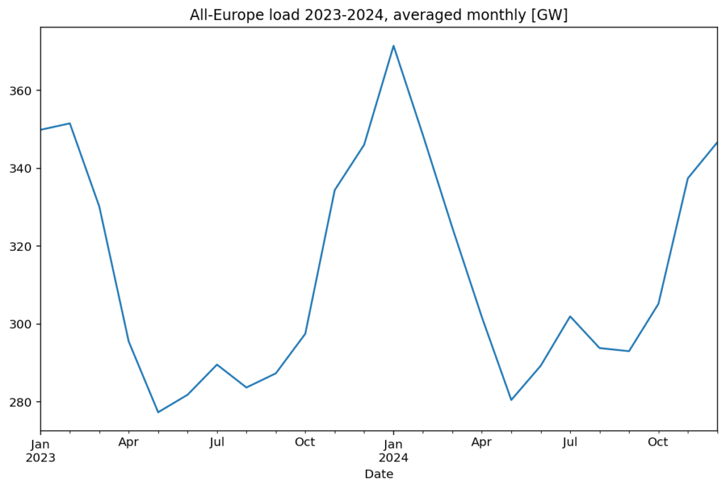
Now, let’s compare this to the load used in the model. The actual electricity load for Europe in 2023–2024 fluctuated between 280 and 360 GW on average (monthly smoothed), i.e. a seasonal swing of around 80 GW. Scaling this load by a factor of 1.5 increases the seasonal variation by around 40 GW, which is significantly less than the 76 GW we estimated for heating electrification.
Conclusion:
The linear scaling used in this model results in a conservative estimate of future seasonal variation. It likely understates the true seasonal swing that will result from converting building heating from fossil fuels to electricity. If biomass-based heating were also replaced by heat pumps, the seasonal variation would increase even further.
För svenskspråkiga läsare finns en förkortad version av den bloggen publicerad på nätforumet Second Opinion: https://second-opinion.se/fossilfritt-europa-2050-tva-scenarier/