
Bengt J. Olsson
Twitter: @bengtxyz
LinkedIn: beos
When things get complicated, it is generally a good idea to try to simplify. A very complex system is the power system. Here’s a very simple balance model of a future Swedish power system modeled in Excel. The model uses “days” as the time unit to keep it more manageable, instead of hours. This also means that there is some inherent flexibility since both production and consumption are “smoothed” over 24 hours. Data is taken from Energy Charts (that is, ENTSO-E) and averaged over 24 hours. Onshore wind, nuclear and load data is taken from Sweden 2023. Due to lack of Swedish data for offshore wind and also rather little statistics for solar, these data are taken from Denmark 2023 instead. Nuclear in Sweden in the beginning of 2023 had an unusually low capacity factor due to reactor problems, so the data have been modified slightly to get the 85% capacity “form factor.”
The installed power values can be scaled. To balance the must-run sources (wind, solar, and nuclear) against the load, mainly reservoir hydropower is used. If hydropower cannot balance to zero, import or “backup” is used. “Backup” can be any flexible power source, such as gas turbines, for example.
Thus, we have three explicit flexibility sources: hydro, import, and backup. These have increasingly higher marginal costs and are thus dispatched in that order: hydro first, then import, and last possibly backup. As mentioned before, there is also an implicit flexibility that could, for example, be constituted by utility battery storage or EV charging that, in essence, smooth out the daily variations. In the dashboard view below, the variation in load is due to the weekend and holiday dips in consumption.
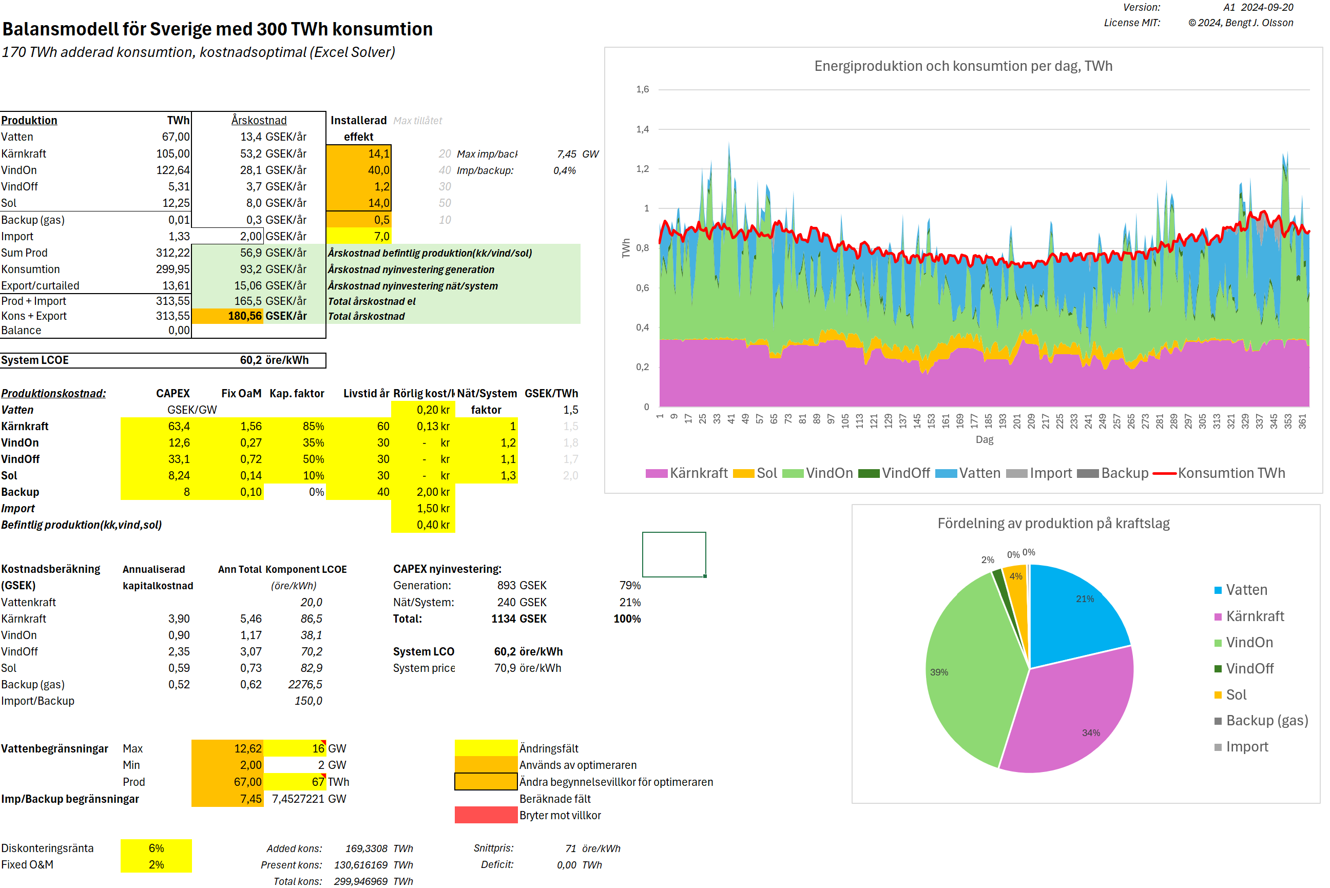
All power sources are assigned production costs and other parameters that provide an annual production cost and LCOE. The costs for Nuclear, On/Offshore wind, and Solar were taken from the NREL Annual Technology Baseline (ATB) database for the year 2040, subject to an exchange rate of 1 USD = 10 SEK. Costs for hydro, import, and backup are my own estimations (that can be changed in the model). The total annual cost divided by the yearly consumption becomes the System LCOE. The built-in non-linear Solver in Excel is used to find the system configuration that provides the minimum annual cost (or System LCOE), given several boundary conditions.
One of these boundary conditions concerns hydro, and it is modeled like this: The hydropower in Sweden can cycle between 2 and 13 GW in power output and produce around 60-70 TWh of electricity per year, depending on the water inflow to the reservoirs. Now, Sweden has 3 GW of import capacity from Norway, from which it can import hydropower. In a “borderless” sense for electricity trading, we can count this as Swedish hydropower. We typically have a net import of 7 TWh from Norway. To not rely too much on hydro, we use the lower limit of the Swedish hydro supply, 60 TWh. Thus, we model the hydro system as a 2-16 GW system that can sustain 67 TWh. Since Swedish hydropower is depreciated a long time ago, a low cost of 20 öre/kWh is assigned to hydropower.
When hydro cannot balance production against load, import is dispatched. This is imagined to happen when the residual load is really high, and the import price can be expected to be high as well. Here it is set to 150 öre/kWh. Note that in a real case, hydro would be exchanged for import during certain hours; hence, import is underestimated here. Sweden have about 10 GW import capacity, but since 3 of these are allocated to the Norwegian hydro import as described above, 7 GW is used for all other import. As a last resort, the solver can build out up to 10 GW of backup capacity (at 8 GSEK per GW, corresponding to gas peakers). The variable cost for this backup capacity is expected to be 200 öre/kWh.
Now the model has two other features as well. First, it counts only additional power capacity and provides the energy level we have today at a fixed “average” price which is set to 40 öre/kWh here (1 SEK = 100 öre). So we start with today’s power system and minimize the cost for building the additional capacity.
The second feature is that it includes an “overhead” cost for network and system costs as well. This is quite speculative but follows a simple model: The total network/system cost investment is assumed to be on the order of 15-30% of the generation cost, depending on the configuration. Now, if we distribute the cost over the power production, the following keys are used. Nuclear is assigned a factor of 1. Offshore wind will probably need slightly more network and system resources, so it is assigned a factor of 1.1 or 10% higher than for nuclear. With the same reasoning, 1.2 and 1.3 (20% and 30% higher than nuclear) are assigned to onshore wind and solar. Then these factors are scaled with a common scale factor to get to about 20% of generation costs in total. This scale factor was set to 1.5, giving the following overhead costs for each power technology:
- Nuclear: 1.5 GSEK/TWh
- Offshore wind: 1.7 GSEK/TWh
- Onshore wind: 1.8 GSEK/TWh
- Solar: 2 GSEK/TWh
Note that the overhead is given per produced TWh, not GW of installed power. The latter would strongly disfavor especially solar with its low capacity factor.
A really cool feature is that it uses the built-in non-linear solver in Excel. In recent versions of Excel, it uses a cloud-based solver that imports the model and uses some powerful methods to do the optimization. Since all non-linear solvers may have difficulties finding the global minima (and not get stuck in local minima), the following strategy is used: For each configuration case (only differing in the boundary condition of how much onshore wind power could be built), two runs were made. The first run used the standard LSGRG non-linear engine, with the “multistart” option. The latter means that it tests different starting points to avoid local minima. Then a run with the standard evolutionary engine was used. These two engines work in very different ways. So if they converged to approximately the same solution, we can conclude that the real cost minimum was found with a high degree of confidence. And they actually produced very similar solutions!
Now, this is a very simplified model of a real system, but the strength is that you can modify it easily and run it in under 1-minute cycles and see what happens. So let’s discuss some of the outcomes.
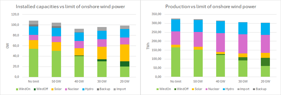
- The solver clearly preferred onshore wind. Without any limitations it would build out 54 GW of onshore wind power. This is 3.5 times the present build-out (16 GW). It may be politically difficult to build so much land based wind power, given the resistance from the people living close to these. The strategy thus became to run a number of simulations where the build-out of onshore wind power was limited. Above is shown the cost optimized production results.
- Also build-out of nuclear (from present 6.9 GW) is preferred in all scenarios, from 3.1 to 7.5 GW depending on limit for onshore wind.
- Offshore wind is sparingly built out. When onshore wind is limited it seems like nuclear is built-out to a certain degree before a combination off offshore wind and solar sets in.
- A solar build-out to 14-32 GW installed capacity, providing between 4-9% of the consumed energy.
- Hydro is always producing its maximum 67 TWh. Not surprising with a low cost of 20 öre/kWh assigned to this depreciated power source.
- Import and backup are quite low in all cases. When the share of renewables is high the import and backup becomes power limited. With nuclear it is possible to import higher volumes with the same import power capacity.
- Export and curtailment varies from 4 to 25 TWh, increasing with higher share of renewables.
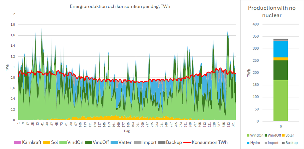
Below is also a hypothetical case with no nuclear. This means more renewable, import, and backup power. Import is power-limited to 6 TWh, and another TWh is produced by 10 GW backup (gas peakers or similar). 38 TWh is exported or curtailed, depending on export capacity. The System LCOE jumps up about 36%, but this is a natural effect of replacing existing depreciated nuclear with new renewables. It costs to turn off existing capacity…
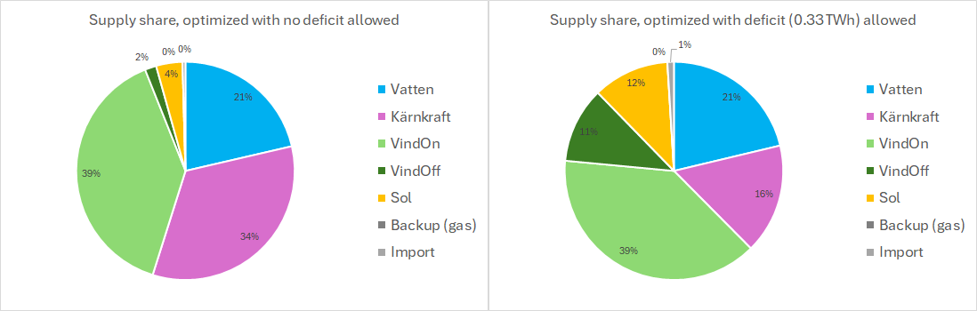
An interesting finding was how sensitive the optimal solution is to deficits. If we allow deficits by removing the last condition, that is that the production deficit (before backup) should be less than what backup can provide, we get a completely new optimal configuration. Let’s look at the 40 GW limited onshore wind production case.
The original optimization, not allowing any deficit, provides a solution with about 14 GW nuclear and little offshore wind and solar (left diagram below). If we instead relax the backup condition, the solver instead sets backup to zero, takes a deficit hit on 0.33 TWh and provides a very different configuration with no nuclear build-out and instead much more offshore wind, solar power and import. The system LCOE is lowered almost 1 öre for this solution (from 60.2 to 59.3 öre/kWh). However, if the needed 5.95 GW backup is added back to this solution, to eliminate the deficit, the system LCOE instead becomes 60.7 öre/kWh, which is more than in the original solution (which of course is right since it now is not an optimal solution).
It is certainly possible to find some kind of flexibility that can handle this 6 GW / 330 GWh deficit, but this flexibility would cost money, and most probably it would not longer be the optimal alternative (as we saw with the gas peaker flexibility above). But we can also see that system cost “hyper-surface” have many local minima with almost the same cost, but corresponding to very different system configurations.
Below is production and cost data for all simulations gathered.
| Limit onshore wind power | ||||||
| No limit | 50 GW | 40 GW | 30 GW | 20 GW | No nuclear | |
| Production/Consumption TWh | ||||||
| Hydro | 67 | 67 | 67 | 67 | 67 | 67 |
| Nuclear | 74 | 83 | 105 | 107 | 101 | 0 |
| WindOn | 166 | 153 | 123 | 92 | 61 | 170 |
| WindOff | 0 | 0 | 5 | 19 | 46 | 82 |
| Solar | 15 | 15 | 12 | 21 | 28 | 13 |
| Backup | 0 | 0 | 0 | 0 | 0 | 1 |
| Import | 3 | 2 | 1 | 1 | 1 | 6 |
| Consumption/Load | 300 | 300 | 300 | 300 | 300 | 300 |
| Export/curtailed | 25 | 21 | 14 | 7 | 4 | 38 |
| Balance | 0 | 0 | 0 | 0 | 0 | 0 |
| Build-out costs GSEK (Miljarder kronor) | ||||||
| Generation: | 822 | 842 | 893 | 964 | 1054 | 1291 |
| Network/System: | 269 | 260 | 240 | 227 | 221 | 372 |
| Total: | 1091 | 1102 | 1134 | 1192 | 1274 | 1664 |
| System LCOE öre/kWh | ||||||
| System LCOE | 60 | 60 | 60 | 61 | 63 | 83 |
To conclude, a total (additional) cost model of a future Swedish power system, including both generation and network/transmission, is made in Excel. Naturally, the model format contains may simplifications and assumptions, but many of these can easily be changed in the sheet.
A 300 TWh system requires between 1100 – 1300 GSEK in build-out costs out of which 17%-25% are network/system costs. The System LCOE is around 60 öre/kWh. This should probably be seen as a lower limit, since there are costs not accounted for in this model. Also the generation costs in the ATB for 2040 are quite a bit lower than todays costs.
The actual System LCOE for the different alternatives varies very little. From the cheapest alternative (no limit on onshore wind) to the most constrained alternative, the difference is only 3.4 öre/kWh or 5.6%. This small difference would likely fall within any possible error bars on the results. The conclusion from this is that we should not necessarily focus solely on the LCOEs or System LCOE. We could also see that by allowing for new kind of flexibilities we could have completely different system configurations with almost the same System LCOE. Thus System LCOE should only be considered as part of the decision basis. Other decision criterias, such as security of supply and system stability must weigh in heavily in the system configuration decision.
A typical system configuration is around 30% nuclear, 40% wind, 22% hydro, 7% solar and less than 1% import an backup. Unfortunately “Others” or biomass and waste thermal generation is not included in this model, it would have had a 3-5% share. The 40 GW onshore wind scenario has some resemblance to the “Elektrifiering Planerpart”, EP, scenario from SvK, see this earlier blog.