SWIS – Western Australia – 2034 SWB system

Bengt J. Olsson
Twitter: @bengtxyz 
LinkedIn: beos

Model
– Generation
– Load
– Hydrogen production
Simulation
– Battery
– Battery + fossil gas
– Battery + green hydrogen
Conclusions
Updates
– Storage for gas backup
– System LCOE for the alternatives
– Cost optimized scenarios
– “Sensible” gas usage scenarios
– Using only hydrogen for backup
Final summary

---

Reading tip: This long blog post has gained a rather convoluted structure with updates added several times… Suggested is maybe to start with the “Final Summary” and work backwards from there.

---

This LinkedIn post spurred a great deal of interest so I’m putting it here as a blog post also with some more detail: https://www.linkedin.com/posts/beos_wind-solar-battery-activity-7217099047092817920-5J9r

Here I investigate the properties of a Solar, Wind and Battery (SWB) system to power the South West Independent System (SWIS) in Western Australia (WA) in 2034. SWIS is particularly interesting is some respects

• It is an isolated power system without import/export possibilities
• It is small enough for at least considering batteries as a firming power source for solar and wind power
• It does not have hydro power or potential for pumped hydro

Essentially, it operates independently, managing the balance between production and consumption. Traditionally, this balance was maintained using fossil fuel power. However, in recent years, solar and wind energy have come to represent approximately 40% of power generation and consumption, with fossil fuels providing both base load and balancing power.

The Australian Energy Market Operator (AEMO) annually publishes an “Electricity Statement of Opportunities” (ESOO) for the Wholesale Electricity Market (WEM). The latest edition includes various demand scenarios, among which the “Expected” scenario is of particular interest. According to this scenario, the anticipated consumption 2034 is projected to be around 35 TWh, with 2 TWh allocated for hydrogen production. This an increase from the current level of approximately 20 TWh.

Model

In this model we investigate how to meet the demand 33 TWh + 2 TWh flexible hydrogen production with 3 sets of generation/storage solutions

• Wind + Solar + Battery
• Wind + Solar + Battery + Gas (fossil)
• Wind + Solar + Battery + Gas (green hydrogen)

In the first part of this long blog post, no lowest total cost optimization is performed, we rather lock in some parameters and vary the others until we have some sort of balance. For example, it will be assumed that the production (in TWh) of wind and solar energy will be the same. This is the case today where both solar and wind production hoovers around 3.5 TWh (each). Since solar has a smaller capacity factor than wind you must build more installed capacity to get the same energy production. But on the other hand, solar PV power is cheaper to build vs wind power, so the assumption of equal energy may be OK, at least for this experiment.

In the “Updates” section we also perform cost optimizations, giving a rather different power system mix.

Generation

The model uses hourly wind and solar data for 2020 to 2022 that @IntermittentNRG (Twitter/X) kindly has provided. This data is normalized to the levels of 2022, to form a consistent base set over three years. Then this normalized data is simply scaled to provide the requested future energy generation.

The model balances must-run generation sources against and load and flexible sources. SWIS is fortunately a rather simple system in this respect. Since SWIS does not have any import/export flexibility, nor variable hydro production, these “degrees of freedom” disappears, and it is possible to have a fixed dispatch merit order. The different sources are:

• Must-run
  • Solar PV
  • Onshore Wind
• Balance
  • Hydrogen production (small impact in this case)
  • Battery (charge and discharge)
  • Fossil gas turbines (only generation)
  • Hydrogen CCGT (only generation)

The battery storage is modelled as fixed size storage with a charge-discharge round-trip efficiency of 85%. Hydrogen storage is also modelled as fixed size storage with an RTE of 35% for hydrogen for CCGT and with no loss for hydrogen production flexibility. Fossil gas power is modelled without a store, that is it is assumed that gas fuel will be available as needed.

Load

Load is modelled to capture the following features that can be seen on the consumption in the OpenNEM graphs. A summer maximum by Jan-Feb and a slightly lower winter maximum in Jul-Aug, and corresponding minima at spring and autumn. To also model a flexible demand that strives to utilize the solar power peak around noon, a daily variation is added, also as a sinus wave, with maximum at noon and minimum at midnight. The seasonal variation is 1 GW peak-to-peak and to this is a 1 GW p-t-p daily variation added which gives a load function that looks like this

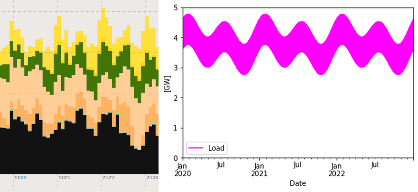
With some fantasy you can identify the summer and winter peaks in the OpenNEM graph to the left. If the Load is summed over all hours of the year we get 33 TWh. (The 2 TWh of flexible gas production is variable and will be added while running the balancing).

Hydrogen production

Hydrogen production constitutes 2 TWh out of the 35 TWh total consumption. This production is made flexible in this way:
Nominal production is 2/8.76 = 0.23 GW. An electrolyzer size of two times the nominal power consumption is chosen, that is 460 MW electrolyzer capacity (thus working at 50 % utilization). A steady delivery of 0.23 GW hydrogen is required. Hence a hydrogen store is required. We have chosen it to be a smaller buffer store of 3 GWh. Now, more than the nominal amount of hydrogen is produced when we have over-capacity, that is by using energy that otherwise should be curtailed. Oppositely if we have lesser energy than required for nominal production, hydrogen is drawn from the store instead of being produced, and thus lower the load. If the store is empty the nominal amount must be produced each hour. At all hours, the nominal amount of hydrogen must be delivered.

This is a simple algorithm that maximises the utility of flexible hydrogen production for this relatively simple system. In reality production of hydrogen would be controlled by the actual price of electricity. But since we don’t model pricing here, the algorithm acts like a “proxy” for this mechanism. (It is likely that electricity would be cheap at negative residual load and hence more produced then, just like in the algorithm above. And vice versa when electricity is scarce).

Hydrogen production for combustion in CCGTs is using the same store, but is with-drawing more gas when used for combustion in order to model the 35% round-trip efficiency.

Simulation

Battery flex only

So let’s start to investigate the first SWB only scenario. We have two parameters to decide, the solar + wind generation and the battery storage capacity (in GWh). We will assume that the battery have the required charging and discharging capacities. By some iterations it is found that a lot of battery capacity is needed if you don’t want to have an absurd overproduction of solar and wind power. So I zoomed in on this distribution

• 38 + 38 TWh of solar + wind power production
• A 100 GWh battery

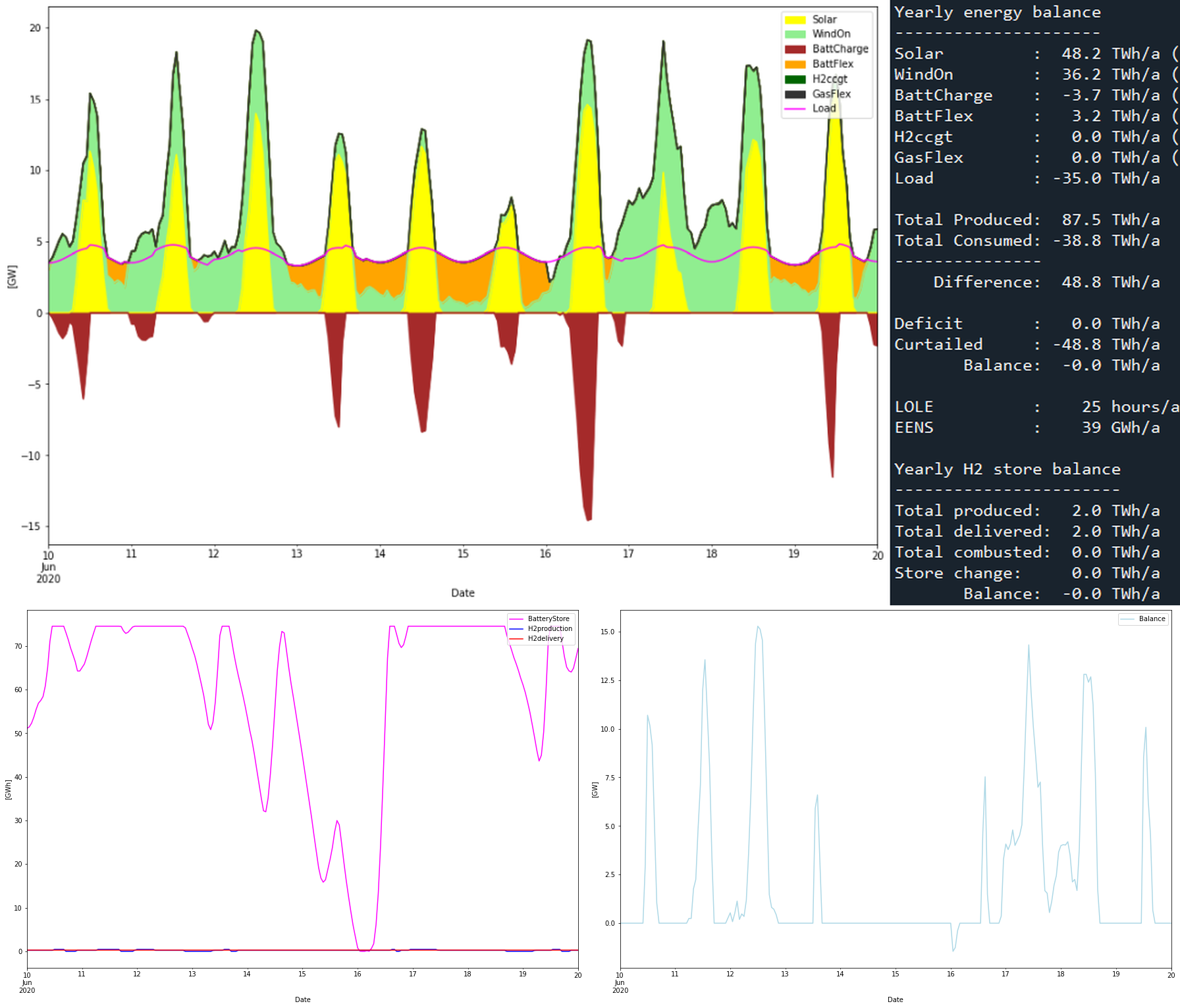
38 + 38 TWh is about 10 times more than todays production of both solar and wind power. I’m not sure about the exact capacity factor on the SWIS scale for solar or wind, but let’s assume 25% and 45% respectively. Then 38 + 38 TWh would correspond to roughly 17 GW solar and 10 GW wind power installed capacities. The 76 TWh of generation is 217% of the 35 TWh consumption, or an overproduction of 117%. The results from the simulation is depicted in the graph below (click it to enlarge).

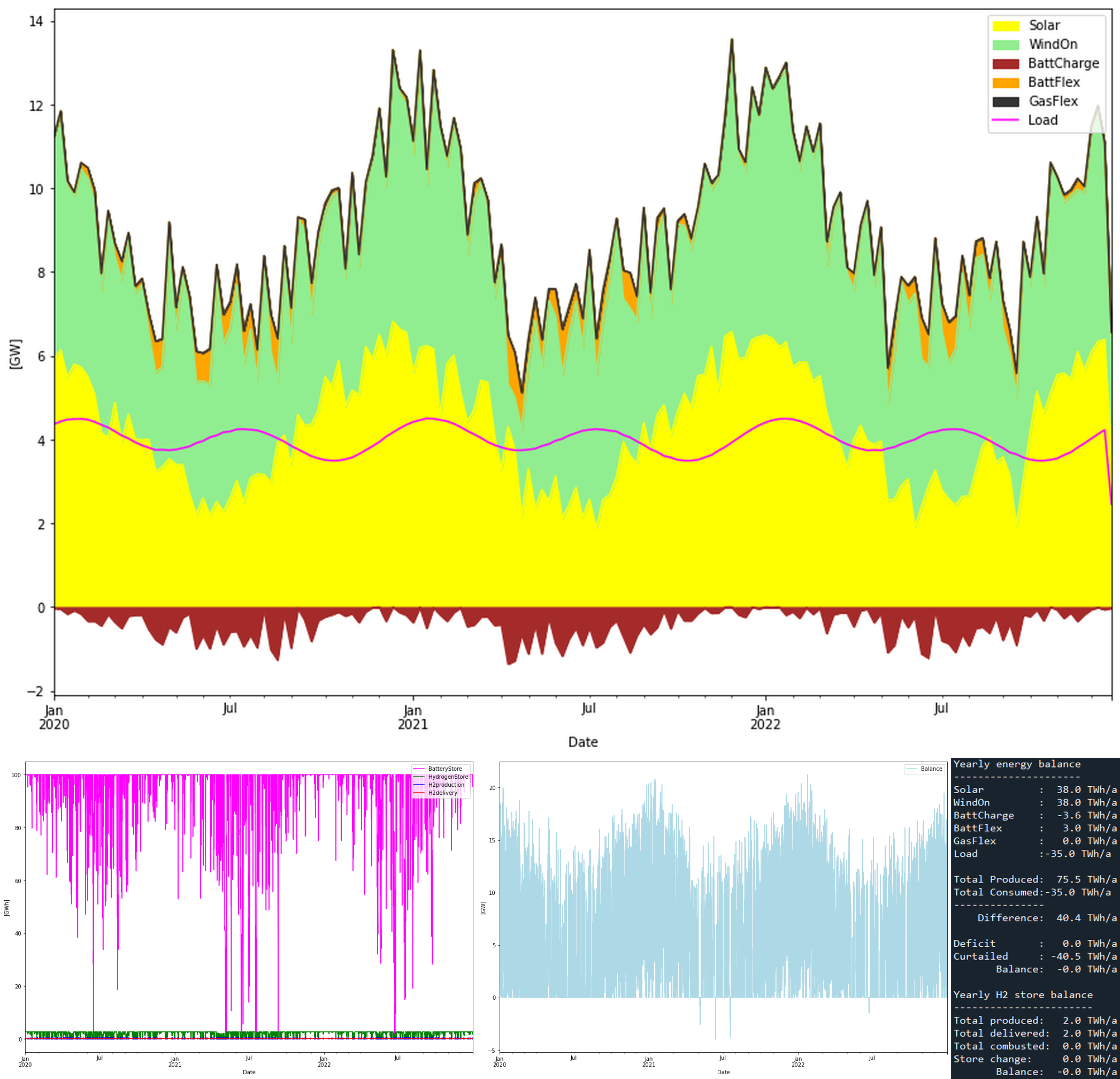
The battery store features seasonal variations where more battery power is needed in the winters. This may sound un-intuitive since the consumption is largest in the summers according to the load curve. But the reason is that in winter the solar PV production is lower and this out-weighs the lower consumption in the winter. (Indicating that maybe more wind than solar in the mix would be better?) Battery charge/discharge is at maximum 14/4 GW, making the battery a 25 hour battery, with respect to discharge.

The negative blue spikes in “Balance” graph shows that we actually have a deficit there. Let’s expand around one of these deficits to see whats happens.

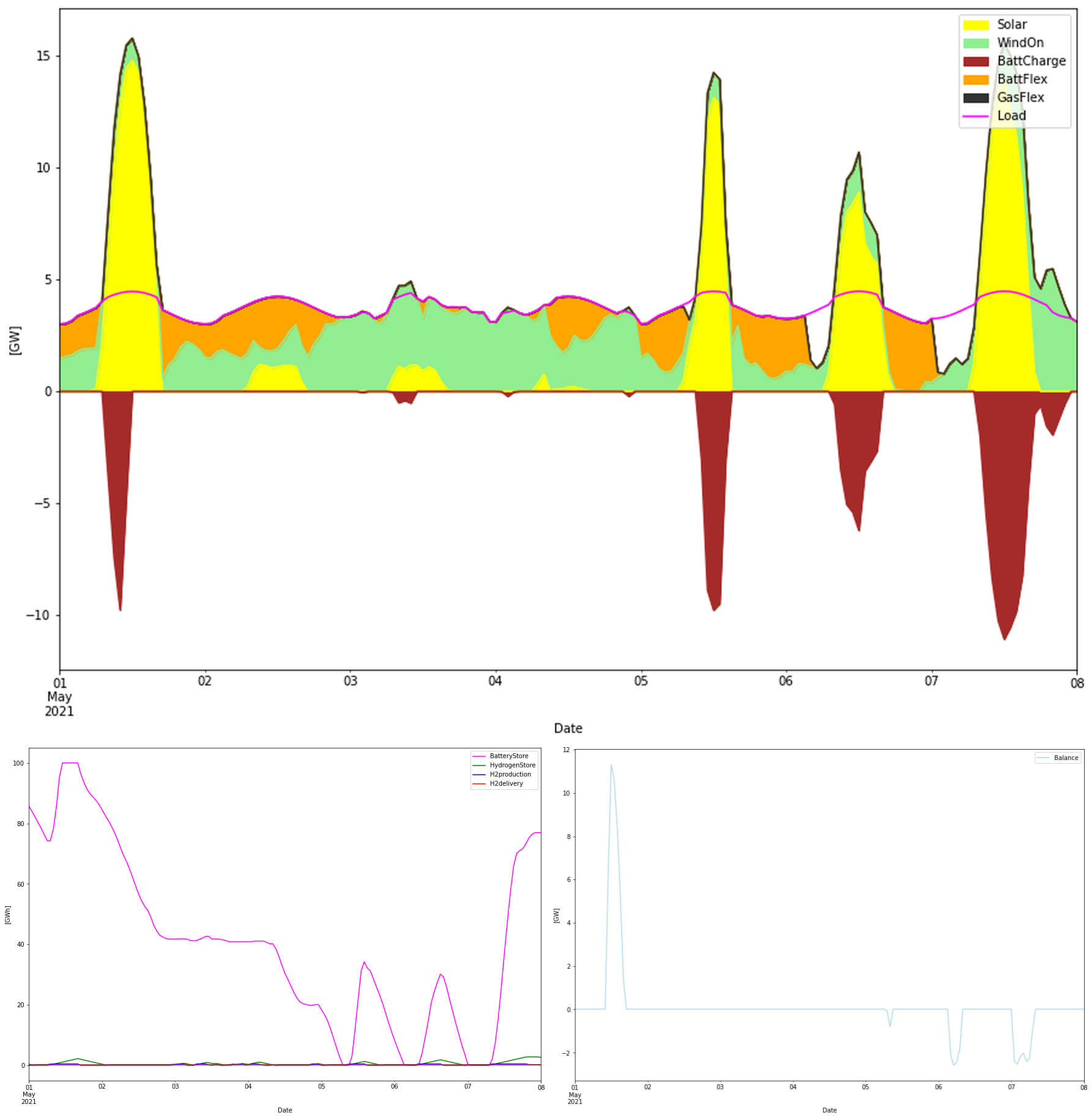
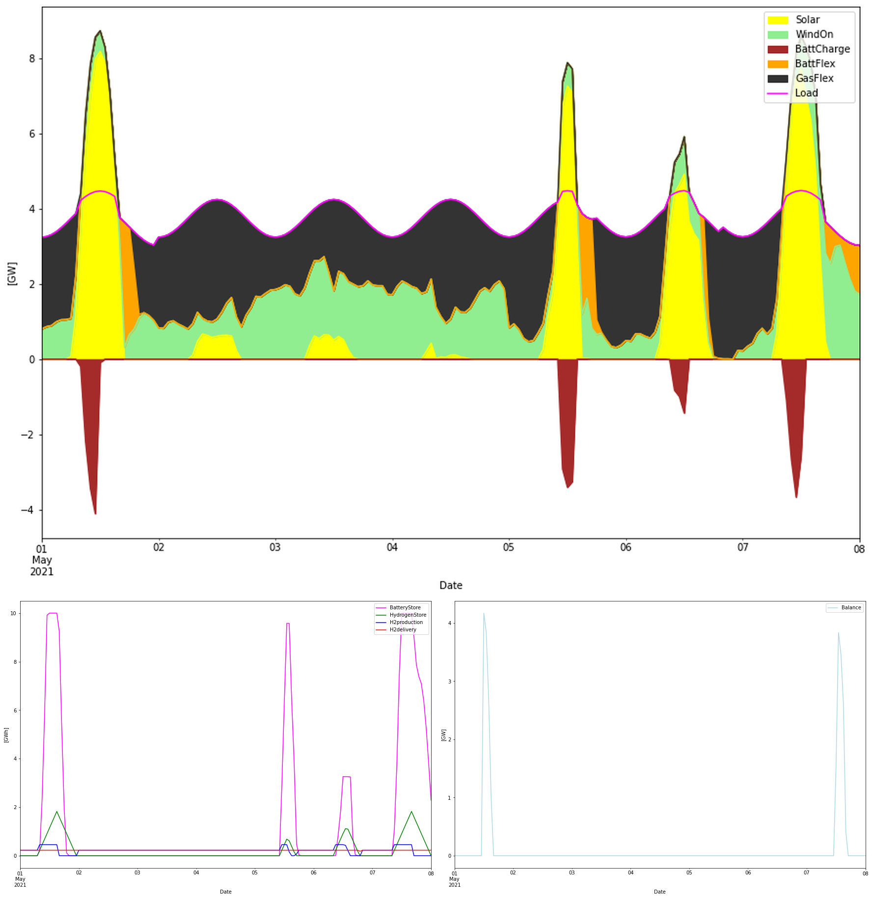
The graph expands the first week of May 2021. Starting out with a fully charged battery May 1, a couple of days with low winds an no sun empties the battery storage and a deficit (white area below load line on top graph, or negative balance in the lower right graph). 100 GWh can thus rather quickly be depleted.

The flexible hydrogen production helps to balance the power, but the effect is too small to really make any difference. As seen in the model section above, hydrogen flexibility can decrease the load with 0.23 GW as long as there is hydrogen in the store. However the 0.23 GW and small store of 3 GWh does not help much against the deficits.

Battery + Gas flex

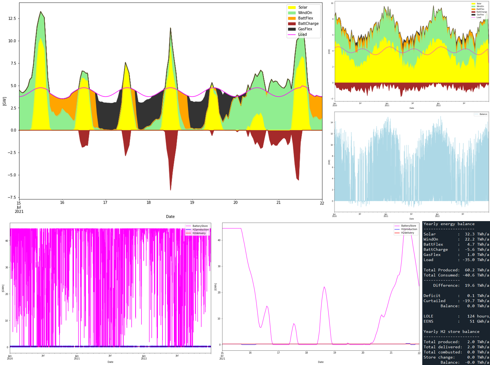
As we could see above, there is a chance that the battery would be depleted almost independent of its size. This since you can never know how long a “dunkelflaute” may last. So a backup mechanism will always be needed in a SWB system. For WA it would be natural to use gas for backup. So let’s model a more realistic system for SWIS where we decide that the RE production should be 120% of the consumption and that the battery store should be 10 GWh (or 3 times larger than the currently largest battery in the world, Moss Landing in California). And that what is further needed in flexibility is handled by natural gas plants with unlimited supply of fuel.

Thus we have

• 21 + 21 TWh of solar + wind power production
• A 10 GWh battery store
• 5 GW of natural gas power plants

to serve the 35 TWh consumption. That is 6 times more solar and wind power than today. In the simulation it will look like this:

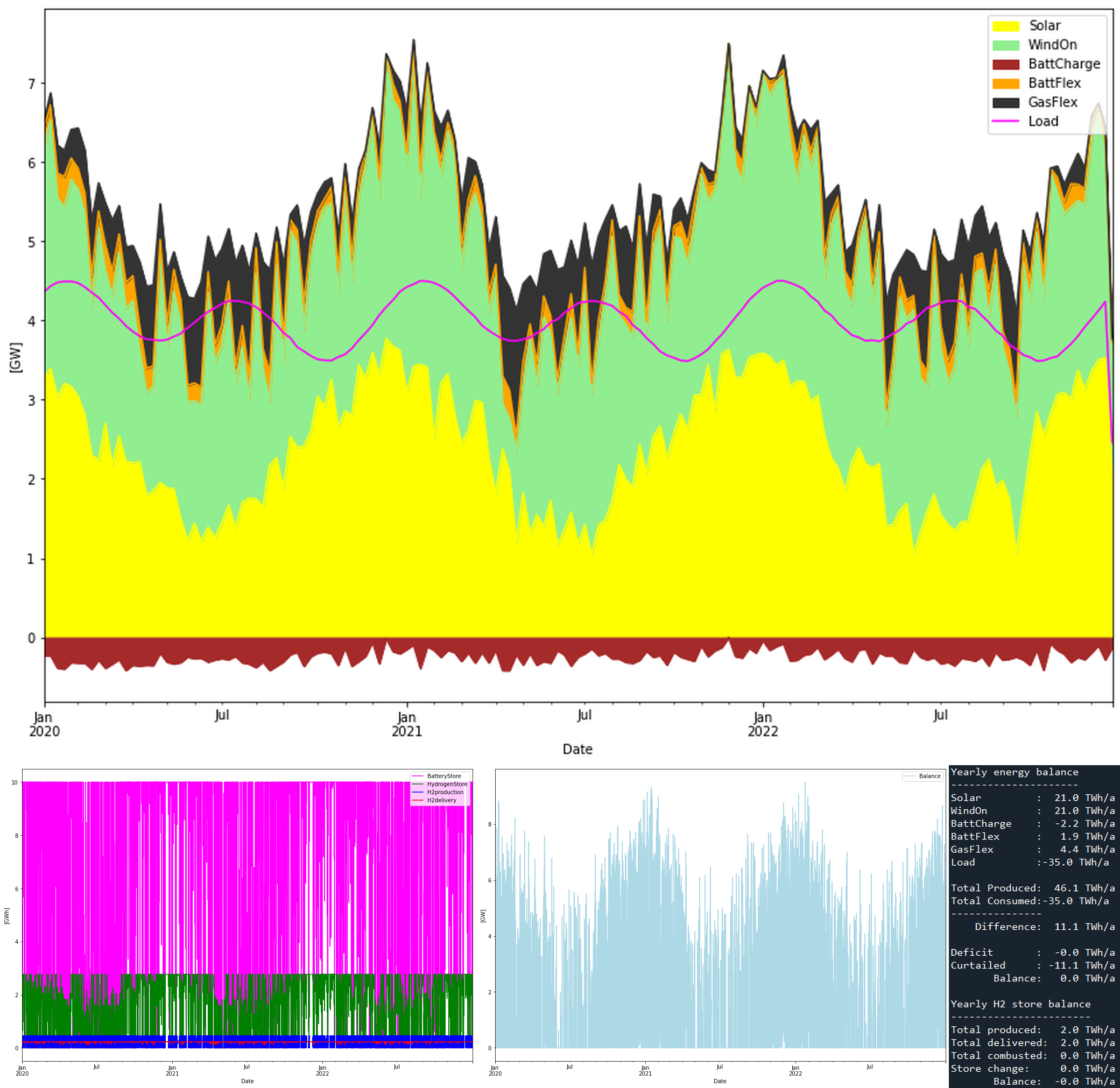
This system has no deficits (lower blue “Balance” graph) as would be expected when gas in principle could supply the system alone. Here, gas comes in at 4.4 TWh out of the 35 TWh consumed, or 13%. 11 TWh of energy is curtailed which is much lower than the 40 TWh in the battery only system (that had a much higher overproduction). Battery charge/discharge is at maximum 6/4 GW, making the battery a 2.5 hour battery. Let’s look at the first week in May, 2021, again:

Gas is used extensively to balance the power system. Battery typically amounts to handle some post-solar hours (as today). It is obvious that gas is needed “to save the day” in this system.

Battery + Hydrogen CCGT flex

What about replacing natural gas with green hydrogen instead? By installing more electrolyzer capacity and 4-5 GW of hydrogen ready combined cycle gas turbines. Then we would get at truly green system without excessive amounts of batteries. Now again we have to fix some parameters. Here is what we chose:

• 31 + 31 TWh of solar + wind power production
• A 10 GWh battery store
• 4 GW of hydrogen ready CCGT power plants
• 14 GW of electrolyzer capacity
• A 1 TWh hydrogen store (!)

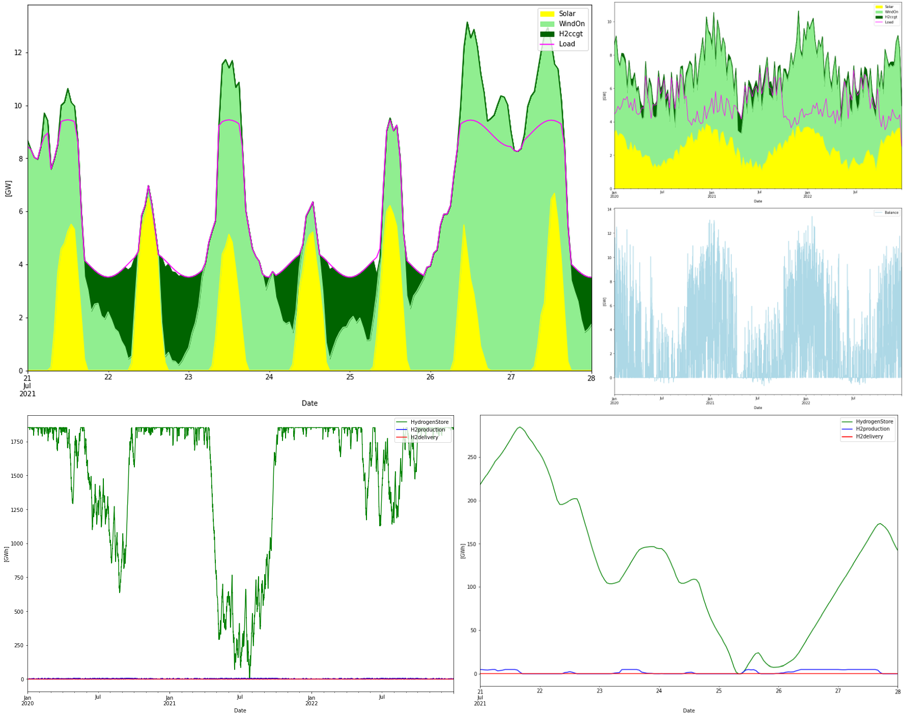
The 1 TWh hydrogen storage size was chosen as a fixed parameter. The 31 + 31 TWh RE production is required to make enough energy for balancing hydrogen fuel. This means 77% of overproduction compared to the 35 TWh consumption. The reason for using CCGT instead of OCGT is that we want to have as high round-trip power->gas->power efficiency as possible. Here we postulate that the RTE with CCGT is 35%. For everything to balance 4 GW of CCGT power and 14 GW of electrolyzer capacity is needed. Electrolyzers are working at 7% utilization.

The merit order of charging and power dispatch is as follows

Charging:

1. Batteries
2. Hydrogen production

Power dispatch

1. Solar + Wind
2. Batteries
3. Hydrogen CCGT

The following simulation results were obtained:

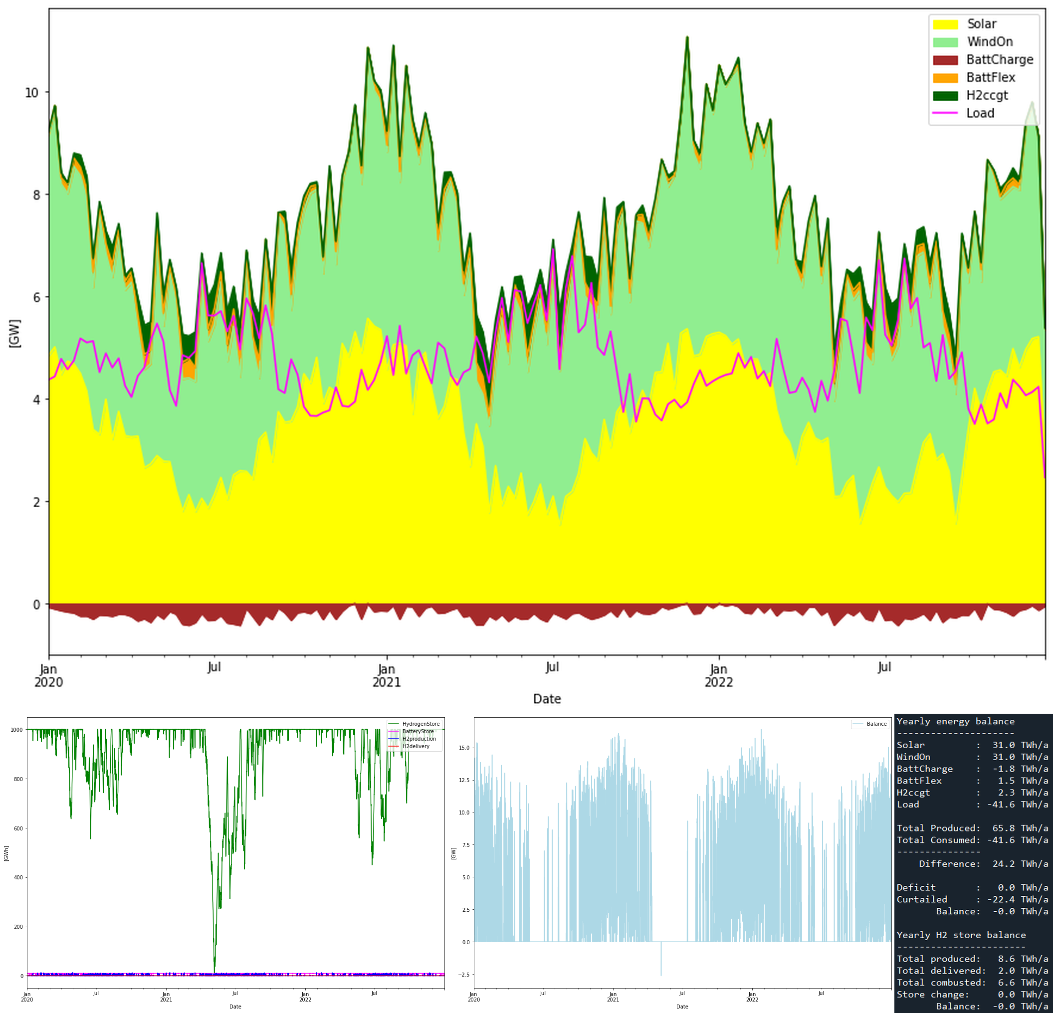
The storage graph is completely dominated by the storage levels of the hydrogen storage, which shows a similar “winter-dip” pattern as in the all-battery case. There is a slight deficit seen in the blue balance graph, in April 2021, that coincides with depletion of the hydrogen storage. But it is so small that we can dismiss it.

From the energy balances we see that 2.3 TWh of hydrogen power is dispatched. In order to do that 6.6 TWh worth of hydrogen is produced (in addition to the 2 TWh that should be delivered externally). We can see that this matches the 35% RTE (2.3/6.6 = 0.35). 22 TWh is curtailed.

Again lets expand some interesting interval. Let’s look at the month leading up to the only deficit:

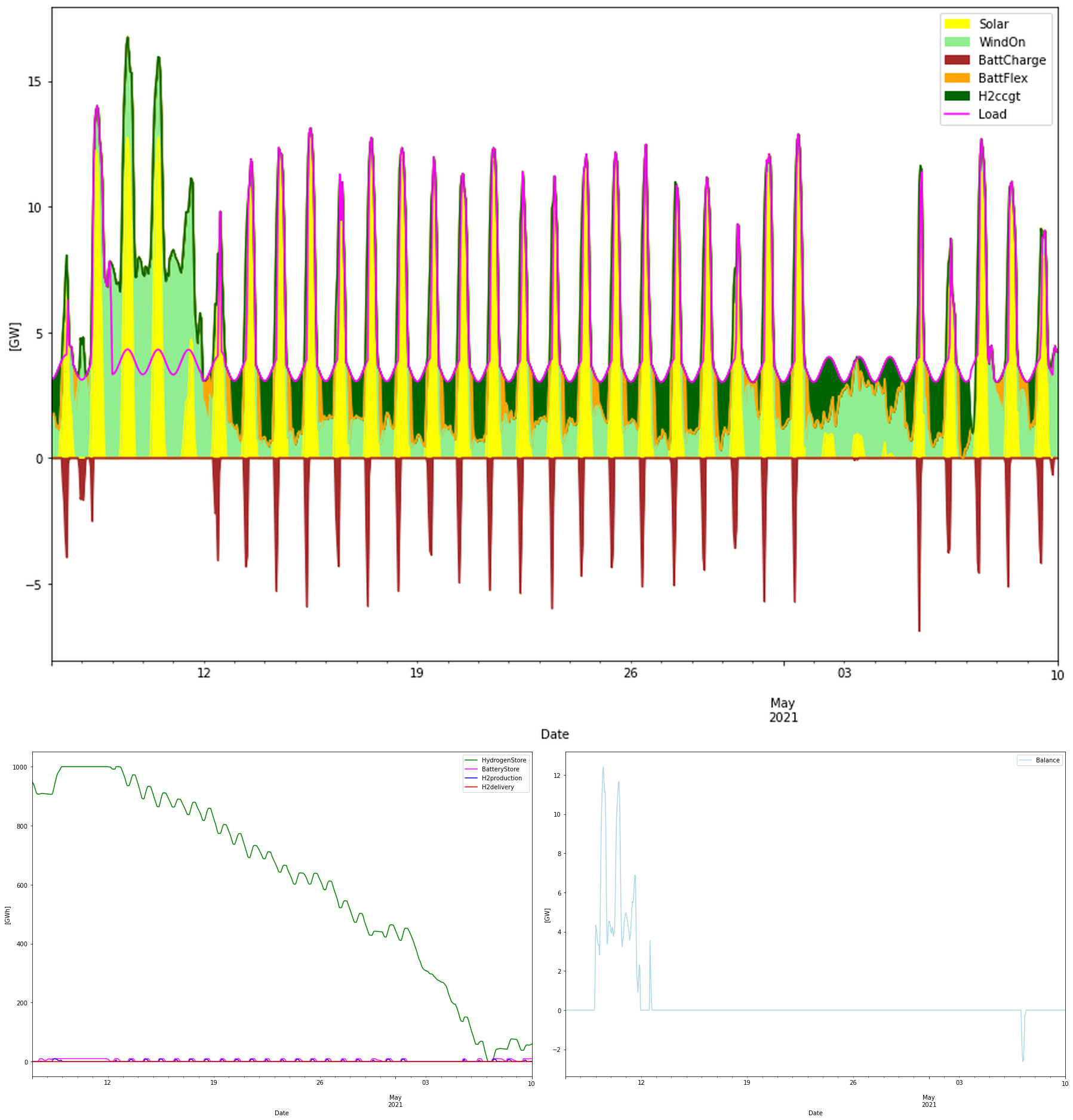
In the beginning of the period both the hydrogen and battery stores are full (lower left), and together with lots of wind and sun, this leads to curtailment (lower right). Then a long wind lull sets in and hydrogen CCGT power is needed to balance. Almost a month of this wind lull drains the 1 TWh store completely and we get a slight deficit at the end of the period.

Conclusions

SWIS in Western Australia is an interesting power system. It is a isolated power system, without import or export. There is plenty of wind and sun in WA, but limited access to hydro power (that is, large scale balancing power). The relatively few degrees of freedom the system has when it comes to balancing makes it a very nice system to model. There are the must-run sources wind and solar power and then there is balancing with either batteries, natural gas power, or power from hydrogen gas power plants. Or a combination of these. Other flexibility sources are relatively small, like demand side respons, and can be neglected since we are not looking at short time peak power adequacy. Instead it is the longer time scale, integrated behavior of supply and demand that is most interesting. Short time demand spikes or power deficits are relatively simple to handle compared to the accumulated deficiencies of supply for example.

Batteries is often the preferred measure to balance RE power. But as can be seen here, the amount of battery storage (100 GWh) is completely out of scale for WA. And then we have also an overproduction of wind + solar power of 117%, that is we curtail more than we consume. If we want to decrease the amount of battery storage we then have to increase the solar + wind power production even more, which is also ridiculous.

Thus a pure Wind + Solar + Battery system is out of the question for WA.

The second variation was to use the accessibility to natural gas and use that for backup. Then we could slim both the wind and solar power production as well as the battery to reasonable sizes. With only 20% overproduction and a 10 GWh battery, the system is in balance thanks to the addition of 13% (of the consumption) fossil gas power. While a 6-fold build out of wind and solar power is needed, this seems like the most straightforward solution. But it has the drawback that it is perpetually dependent on fossil fuel backup.

The third variation is to use hydrogen CCGT power instead of fossil gas, to obtain a carbon free power system without excessive battery stores. However, in this system the hydrogen storage instead becomes excessive, 1 TWh in this example. Then we still had to increase the wind+solar energy from 21+21 to 31+31 TWh in order to produce the hydrogen. Also a whopping 14 GW of elctrolyzers are needed, that are utilized to only 7%. All in all this seems like an unattractive solution.

The alternatives seems to be either wind + solar power backed with mainly fossil gas, perhaps partly including hydrogen CCGT / hydrogen store solution to offset some of the fossil gas. It also seems like a greater share of wind power, relative solar, would be beneficial since it is really the seasonal variations of the solar power that is the culprit with respect to energy storage. And this is very hard to do anything about… Or find a way to offset a large part of the variable power with some kind of stable and clean base load power, to minimize the problems with balancing.

Or why not only have say 5 GW of stable clean baseload power (wonder which…? 😉 )that covers all power needs and follow load by using surplus power for hydrogen production…

Updates

2024-07-20 storage needs for gas backup

For the second alternative, RE with fossil gas backup, I used the simple assumption that fossil gas vas available when needed. If we look at this in little more detail, availability of backup gas is not trivial. Like batteries or hydrogen that are used for backup, also gas needs some kind of storage. The energy for this storage is, differently from batteries/hydrogen, not sourced by the power system itself, but from an external source. Nevertheless, a storage is needed since it would be very difficult to source backup gas “just in time”.

The 4.4 TWh of gas needed each year corresponds to an average consumption of about 0.5 GW. (Note that everything is measured in terms of the electric energy the gas produces, which depends on the efficiency of the gas to power conversion. We need to convert this to, for example, LHV value for the natural gas afterwards, in order to measure the storage in actual gas energy units). Let’s assume that we build a gas supply system that can supply 1 GW worth of gas continuosly to a gas storage. It will do that all the time (unless the storage is full). In that case the fill level of the gas store will look like this:

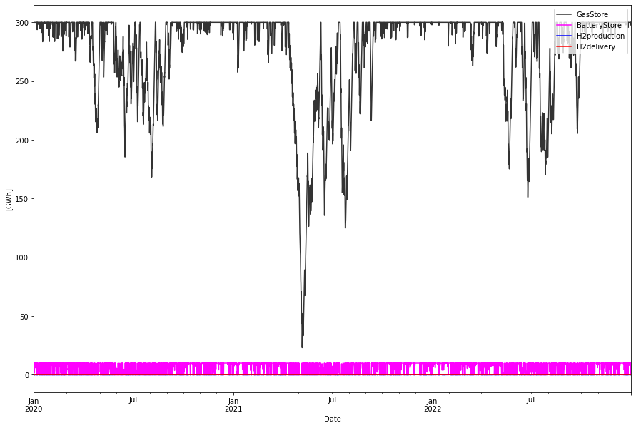
About 300 GWh of storage is needed in this case with 1 GW inflow. Is this much or little? To see this we first have to convert the store units to gas energy units. If we are assuming flexible open cycle gas turbines in this case we have an efficiency of say 40%. Thus the 300 GWh storage becomes a 750 GWh measured as LHV of NG. If the LHV of NG is 13.6 kWh/kg the mass of the stored gas becomes 55 kt (kilotons). If we compress the NG to 200 bar we get a density of about 180 kg/m3, leading to a needed storage volume of about 300.000 m3.

One comparison could be done to the worlds currently largest Lined Rock Cavern (LRC) storage, the “Skallen” storage in the south of Sweden. It has a volume of about 40.000 m3. Thus, WA would need natural gas storages corresponding to 7.5 of the Skallen storage facilities.

Also note that 1 GW inflow would correspond to a 2.5 GW LHV gas flow in this case. The maximum consumption during an hour was about 4 GWh corresponding to a LHV gas flow need that hour of 10 GW. Both 2.5 GW and 10 GW are indeed very high gas flows.

This “back of the envelope” calculation indicate that large scale renewable power production from wind and solar brings in a new problem: Intermittency in backup gas usage, that implies new requirements in the logistics of the gas supply. In particular the need for, probably distributed, energy storages also for this backup medium.

2024-07-27: System LCOE for the three scenarios

Using the CSIRO cost estimates for 2040 and corresponding life times for the different power sources, as well as for storage and gas backup, it is possible to calculate the total cost of the system. The “low assumption” cost alternatives from CSIRO were used where applicable, and the “Global NZE post 2050”, which is the mid alternative, where this was applicable. The total calculated cost is annualized, using a 6% discount rate, and divided by the produced energy that meets the consumption (that is 35 TWh per year). In this way the System LCOE is obtained. The System LCOE internalizes the firming costs that can be hard to etimate when only looking at LCOE for the respective power sources. Network and grid stability costs are not included, this models only look at energy and power balances. Capacity factors of 45% for wind and 30% for solar have been assumed.

The following System LCOE were obtained for the three cases

38 + 38 TWh wind/solar and 100 GWh battery

          Installed Capacity Unit  TWh/year  CAPEX/GW(h)  OPEX/MW(h)/y   CRF  Tot CAPEX  Tot OPEX  Ann Cost    LCOE
WindOn                9.640   GW    38.000        1.871        25.000 0.078     18.036     0.241     1.652  43.471
Solar                14.460   GW    38.000        0.832        17.000 0.073     12.030     0.246     1.120  29.469
H2Store               3.000  GWh     0.000        0.001         0.020 0.066      0.003     0.000     0.000     inf
H2Elys                0.457   GW     0.000        0.489        15.000 0.103      0.223     0.007     0.030     inf
H2ccgt                0.000   GW     0.000        1.702        10.900 0.078      0.000     0.000     0.000     NaN
GasT                  0.000   GW     0.000        0.850        92.200 0.078      0.000     0.000     0.000     NaN
Battery             100.000  GWh     3.137        0.141         1.410 0.103     14.100     0.141     1.593 507.802

Total over-night cost           44.4 BAUD
Total yearly OPEX costs          0.6 BAUD
Annualized cost                  4.4 BAUD
System LCOE                    125.6 AUD/MWh

21 + 21 TWh wind/solar and 10 GWh battery and gas backup

          Installed Capacity Unit  TWh/year  CAPEX/GW(h)  OPEX/MW(h)/y   CRF  Tot CAPEX  Tot OPEX  Ann Cost    LCOE
WindOn                5.327   GW    21.000        1.871        25.000 0.078      9.967     0.133     0.913  43.471
Solar                 7.991   GW    21.000        0.832        17.000 0.073      6.648     0.136     0.619  29.469
H2Store               3.000  GWh     0.000        0.001         0.020 0.066      0.003     0.000     0.000     inf
H2Elys                0.457   GW     0.000        0.489        15.000 0.103      0.223     0.007     0.030     inf
H2ccgt                0.000   GW     0.000        1.702        10.900 0.078      0.000     0.000     0.000     NaN
GasT                  4.176   GW     4.569        0.850        10.200 0.078      3.550     0.417     0.695 152.092
Battery              10.000  GWh     1.954        0.141         1.410 0.103      1.410     0.014     0.159  81.520

Total over-night cost           21.8 BAUD
Total yearly OPEX costs          0.7 BAUD
Annualized cost                  2.4 BAUD
System LCOE                     69.0 AUD/MWh

31 + 31 TWh wind/solar and 10 GWh battery and Hydrogen CCGT backup

          Installed Capacity Unit  TWh/year  CAPEX/GW(h)  OPEX/MW(h)/y   CRF  Tot CAPEX  Tot OPEX  Ann Cost    LCOE
WindOn                7.864   GW    31.000        1.871        25.000 0.078     14.714     0.197     1.348  43.471
Solar                11.796   GW    31.000        0.832        17.000 0.073      9.814     0.201     0.914  29.469
H2Store            1000.500  GWh     2.294        0.001         0.020 0.066      1.000     0.020     0.087  37.712
H2Elys               14.000   GW     2.294        0.489        15.000 0.103      6.846     0.210     0.915 398.848
H2ccgt                4.000   GW     2.294        1.702        10.900 0.078      6.808     0.044     0.576 251.183
GasT                  0.000   GW     0.000        0.850        92.200 0.078      0.000     0.000     0.000     NaN
Battery              10.000  GWh     1.508        0.141         1.410 0.103      1.410     0.014     0.159 105.639

Total over-night cost           40.6 BAUD
Total yearly OPEX costs          0.7 BAUD
Annualized cost                  4.0 BAUD
System LCOE                    114.2 AUD/MWh

Note that the component LCOE values for wind and solar agrees quite well with the CSIRO values at 43 and 28 respectivelly. The other interesting thing we see is that the LCOE for the battery part will depend strongly on the utilization (as can be expected). In the first case with only battery backup it must be so large, and together with a strong overproduction, the battery is not cycled as much as needed to bring down its costs. 3137 GWh/year implies a cycle time of 11.6 days (on average). Each produced battery MWh thus becomes very expensive. The opposite is seen in the second, gas backup case. Here the 10 GWh produces 1954 GWh per year => cycle time of 1.9 days, which is reflected in the correspondingly lower LCOE.

The hydrogen CCGT backup alternative is not as expensive as the battery only backup scenario, but much more expensive than the gas backup scenario. We can see that it is the low utilization of the electrolyzers, as well as for the CCGTs, that drives up the cost.

---

Cost optimized scenarios

All scenarios above have been “hand-crafted”, where certain parameters (for example wind and solar energy production per year) has been chosen and then balancing has been done by testing various balance power parameters. In this section we will instead do a cost minimization, using the costs from CSIRO as discussed above.

Wind, Solar and large Battery

          Installed Capacity Unit  TWh/year  CAPEX/GW(h)  OPEX/MW(h)/y   CRF  Tot CAPEX  Tot OPEX  Ann Cost    LCOE
WindOn                9.179   GW    36.185        1.871        25.000 0.078     17.175     0.229     1.573  43.471
Solar                18.332   GW    48.177        0.832        17.000 0.073     15.252     0.312     1.420  29.469
H2Store               3.000  GWh     0.000        0.001         0.020 0.066      0.003     0.000     0.000     inf
H2Elys                0.457   GW     0.000        0.489        15.000 0.103      0.223     0.007     0.030     inf
H2ccgt                0.000   GW     0.000        1.702        10.900 0.078      0.000     0.000     0.000     NaN
GasT                  0.000   GW     0.000        0.850        92.200 0.078      0.000     0.000     0.000     NaN
Battery              74.536  GWh     3.180        0.141         1.410 0.103     10.510     0.105     1.187 373.388

Total over-night cost           43.2 BAUD
Total yearly OPEX costs          0.7 BAUD
Annualized cost                  4.2 BAUD
System LCOE                    120.3 AUD/MWh

In the this first scenario with only wind, solar and a large battery as backup, the optimization algorithm preferred to overbuild more cheap solar and downsize the battery somewhat. The overbuild is a massive 140% and hence curtailing more energy, 49 TWh, than is consumed. The System LCOE ended up at 120 AUD/MWH, not that far from the corresponding un-optimized scenario (126 AUD/MWh).

Wind, Solar and Battery plus Gas backup

Here we did two sub-scenarios. In the first we vary wind, solar, gas and battery capacities. In the second sub-scenario we keep the battery size fixed at 10 GWh.

Sub-alternative 1: Battery capacity also varied

          Inst. Cap. Unit  TWh/year  CAPEX/GW  OPEX/GW/y  Fuel/y   CRF  Tot CAPEX  Tot OPEX  Ann Cost    LCOE
WindOn        4.568   GW    18.007     1.871      0.025   0.000 0.078      8.547     0.114     0.783  43.471
Solar         3.842   GW    10.097     0.832      0.017   0.000 0.073      3.197     0.065     0.298  29.469
GasT          3.846   GW     9.196     0.850      0.010   0.754 0.078      3.269     0.793     1.049 114.075
Battery       0.044  GWh     0.013     0.141      0.001   0.000 0.103      0.006     0.000     0.001  55.050

Total over-night cost           15.2 BAUD
Total yearly OPEX costs          1.0 BAUD
Annualized cost                  2.2 BAUD
System LCOE                     61.7 AUD/MWh

The battery was almost completely eliminated in this alternative. Gas provides 26% of the consumed energy. With no storage capacity, the optimizer opted to increase wind power capacity. This is anticipated as a lower storage capacity necessitates a steadier power supply, which wind power, unlike solar power, is more likely to provide. Only 2.3 TWh (7%) is curtailed.

Sub-alternative 2: Battery capacity kept fixed at 10 GWh

          Inst. Cap. Unit  TWh/year  CAPEX/GW  OPEX/GW/y  Fuel/y   CRF  Tot CAPEX  Tot OPEX  Ann Cost    LCOE
WindOn        4.330   GW    17.067     1.871      0.025   0.000 0.078      8.101     0.108     0.742  43.471
Solar         5.040   GW    13.245     0.832      0.017   0.000 0.073      4.193     0.086     0.390  29.469
GasT          3.839   GW     7.437     0.850      0.010   0.610 0.078      3.263     0.649     0.904 121.591
Battery      10.000  GWh     1.697     0.141      0.001   0.000 0.103      1.410     0.014     0.159  93.873

Total over-night cost           17.2 BAUD
Total yearly OPEX costs          0.9 BAUD
Annualized cost                  2.2 BAUD
System LCOE                     63.6 AUD/MWh

When the battery capacity was fixed at 10 GWh, the gas usage shrunk to about 20% of the consumption.

The cost of the second alternative is slightly higher (64 vs 62 AUD/MWh) which is expected since we keep one optimization parameter fixed in this case. But both the fossil gas alternatives are almost at half the System LCOE compared to the Battery only alternative (and less than half in CAPEX/investment costs). It will thus be hard to eliminate gas from an economic point of view. Note however, that no explicit CO2 taxes have been added to the fuel cost.

A mixed scenario with both hydrogen CCGT and fossil GT was performed, but the hydrogen CCGT was squeezed out of the optimization due to its high costs (not only the CCGT but also the larger electrolyzers and to some degree, the hydrogen storage). It is not an entirely fair comparison, since no over-head cost have been applied to the fossil gas backup (such as fossil gas storage), but the conclusion would probably the same with these costs added.

“Sensible” Gas usage scenarios

The optimization with and without gas provides to extreme solutions with System LCOE varying from 62 AUD/MWh (gas only, no batteries) to 120 AUD/MWh. The former solution (gas only) provides a “lean” system with only 7% curtailment. This means that the buildout of wind and solar power is manageable, still about 9 times from today. The drawback is of course the perpetualized dependence on natural gas that constitutes 20-25% of the energy supply. In absolute terms, this is the same amount as is consumed today, around 7.5 TWh.

The Battery only extreme is not viable at all. It demands a 75 GWh battery, which is questionable if it is even possible to aquire in the 2034 time frame. Also wind and solar needs to overproduce insame amounts, more energy is curtailed than consumed (140% curtailment). This also means that 24 times the current production of solar and wind power needs to be installed. On top of these drawbacks the System LCOE is almost doubled to 120 AUD/MWh.

So clearly there need to be some intermediate scenario inbetween these two extremes. We can construct such scenarios by postulating fixed amounts of gas turbine capacity. In the gas only scenario the gas turbine capacity naturally matched the maximum demand. With a combination of gas turbines and batteries it is not required to have this much capacity of gas turbines, since the battery can provide ample power as well. So in this mixed model we will fix gas turbine capacity at some max capacities and also continue with the dispatch rule that gas power is produced as a last resort, when all other options are unavailable.

2 GW Gas capacity

Here are the cost optimized results from a wind, solar, battery system with 2 GW gas backup capacity:

          Inst. Cap. Unit  TWh/year  CAPEX/GW  OPEX/GW/y  Fuel/y   CRF  Tot CAPEX  Tot OPEX  Ann Cost    LCOE
WindOn        5.564   GW    21.935     1.871      0.025   0.000 0.078     10.411     0.139     0.954  43.471
Solar        19.604   GW    51.520     0.832      0.017   0.000 0.073     16.311     0.333     1.518  29.469
GasT          2.000   GW     0.181     0.850      0.010   0.015 0.078      1.700     0.035     0.168 931.399
Battery      59.100  GWh     5.189     0.141      0.001   0.000 0.103      8.333     0.083     0.941 181.422

Total over-night cost           37.0 BAUD
Total yearly OPEX costs          0.6 BAUD
Annualized cost                  3.6 BAUD
System LCOE                    103.2 AUD/MWh

Yearly energy balance
---------------------
Solar         :  51.5 TWh/a (70.8%)
WindOn        :  21.9 TWh/a (30.2%)
BattCharge    :  -6.1 TWh/a (-8.4%)
BattFlex      :   5.2 TWh/a ( 7.1%)
GasFlex       :   0.2 TWh/a ( 0.2%)
Load          : -35.0 TWh/a

Total Produced:  78.8 TWh/a
Total Consumed: -41.1 TWh/a
---------------
    Difference:  37.7 TWh/a

Deficit       :   0.0 TWh/a
Curtailed     : -37.7 TWh/a
       Balance:  -0.0 TWh/a

LOLE          :    54 hours/a
EENS          :    47 GWh/a

In this model, a mere 180 GWh of gas facilitates the displacement of over 10 TWh of wind and solar energy, while also reducing the battery capacity requirement from 75 to 60 GWh. This appears to be a highly beneficial trade-off, as the required gas could be sustainably sourced from biomethane or equivalent. Notably, it is predominantly wind power that is curtailed, whereas solar power sees an increase. The system’s Levelized Cost of Energy (LCOE) has decreased from 120 to 103 AUD/MWh, indicating significant economic benefits from this minimal gas consumption.

3 GW Gas capacity

          Inst. Cap. Unit  TWh/year  CAPEX/GW  OPEX/GW/y  Fuel/y   CRF  Tot CAPEX  Tot OPEX  Ann Cost    LCOE
WindOn        5.642   GW    22.239     1.871      0.025   0.000 0.078     10.555     0.141     0.967  43.471
Solar        12.275   GW    32.258     0.832      0.017   0.000 0.073     10.213     0.209     0.951  29.469
GasT          3.000   GW     0.979     0.850      0.010   0.080 0.078      2.550     0.111     0.310 316.982
Battery      44.487  GWh     4.727     0.141      0.001   0.000 0.103      6.273     0.063     0.709 149.911

Total over-night cost           29.8 BAUD
Total yearly OPEX costs          0.5 BAUD
Annualized cost                  3.0 BAUD
System LCOE                     84.8 AUD/MWh

With 3 GW capacity the gas consumption increases 5 times to a total of 1 TWh, or about 3% of the consumption. Removes 20 TWh of solar power, but same wind power as with 2 GW. A 45 GWh battery is still needed, but cost is down with almost 30% vs the battery only case.

Hydrogen store instead of gas/battery backup

In this exercise, wind and solar power is balanced entirely by hydrogen that is produced and stored wnen wind plus solar power is in excess of the demand. And then combusted in a hydrogen ready combined-cycle gas turbine (CCGT). A CCGT is used instead of an open-cycle GT in order to get a not-so-bad round-trip efficiency (RTE). RTE here is assumed to be 0.35 all things considered. That is from making hydrogen out of electricity, compress and store the hydrogen, and finally feeding into a CCGT to get electricity back, 65% of the original electricity is lost. (Compare this with the battery store RTE that is assumed to be 85%). No battery and no fossil gas backup is allowed here. The optimization presents the following results:

          Inst. Cap. Unit  TWh/year  CAPEX/GW  OPEX/GW/y  Fuel/y   CRF  Tot CAPEX  Tot OPEX  Ann Cost    LCOE
WindOn        9.528   GW    37.561     1.871      0.025   0.000 0.078     17.828     0.238     1.633  43.471
Solar         8.222   GW    21.607     0.832      0.017   0.000 0.073      6.841     0.140     0.637  29.469
H2Store    1853.186  GWh     3.273     0.001      0.000   0.000 0.066      1.853     0.037     0.160  48.961
H2Elys        4.931   GW     3.273     0.489      0.015   0.000 0.103      2.411     0.074     0.322  98.465
H2ccgt        3.354   GW     3.273     1.702      0.011   0.000 0.078      5.709     0.037     0.483 147.626


Total over-night cost           34.6 BAUD
Total yearly OPEX costs          0.5 BAUD
Annualized cost                  3.2 BAUD
System LCOE                     92.4 AUD/MWh

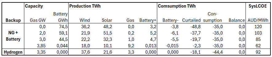
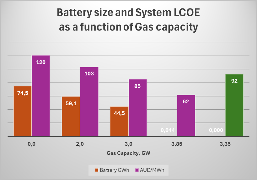
It is evident that some amount of fossil gas will be needed to support the battery backup schemes. As can be seen, the cost quickly increases with the amount of batteries needed. Another problem is probably the sheer scale of the battery need. Say that 800.000 small houses or villas in WA each has 15 kWh in battery storage, that amounts to about 12 GWh. The rest would come from grid-scale battery store. Compare with for example the currently biggest battery storage in the world, Moss Landing in California, which is 3 GWh. WA would need grid battery storage corresponding to 10 – 20 times the size of the Moss Landing facility.

Thus, the Hydrogen alternative becomes interesting as well. 5 GW of electrolyzer capacity, paired with 3.3 GW of hydrogen CCGT capacity and underground hydrogen storage, can balance the system without fossil gas at an intermediate cost (green bar in the graph). Much more gas energy than 4 PJ is stored in underground storage in WA today..

As usually is the case, a combination of natural gas, battery and hydrogen backup may be optimal.

I haven’t come around to try a nuclear base load scenario, but guess that with the extremely high costs that CSIRO GenCost associates with nuclear power, it would be excluded in the optimization. But with somewhat more reasonable prices the situation may be different…