The three-zone market using flow based constraints

Bengt J. Olsson
Twitter: @bengtxyz 
LinkedIn: beos

In earlier posts, we explored a two-zone and a three-zone electricity market, each with different demand and supply curves. By allowing electricity to flow from low-price zones to high-price zones, total welfare was maximized. However, these models assumed perfect flexibility, ignoring the physical constraints of the power network, instead flows were determined solely by economic optimization.

In this post, we revisit the three-zone market and examine how the results change when physical realities, such as network impedances, are taken into account. We also introduce a new concept: a zone-internal congestion point (a.k.a. a “CNEC”). This internal bottleneck can lead to price splitting, and also un-intuitive flows, even when there’s no congestion between zones.

An interesting observation from the three-zone model is that while net positions are uniquely determined by economic optimization, the flows between zones are not. The net position of a zone can be interpreted in two equivalent ways:

• The difference between supply and demand within the zone
• The net export: the sum of flows out of the zone minus the sum of flows into the zone

As long as the net positions of the zones remain the same, there are infinitely many possible flow configurations between them—unless a congestion occurs. (See the previous post on the three-zone model for concrete examples of this.)

In practice, however, only one set of flows will occur. This set is determined by economic optimization, but subject to physical constraints of the power network. Let’s take a closer look at those constraints.

---

Introducing Internal Congestion

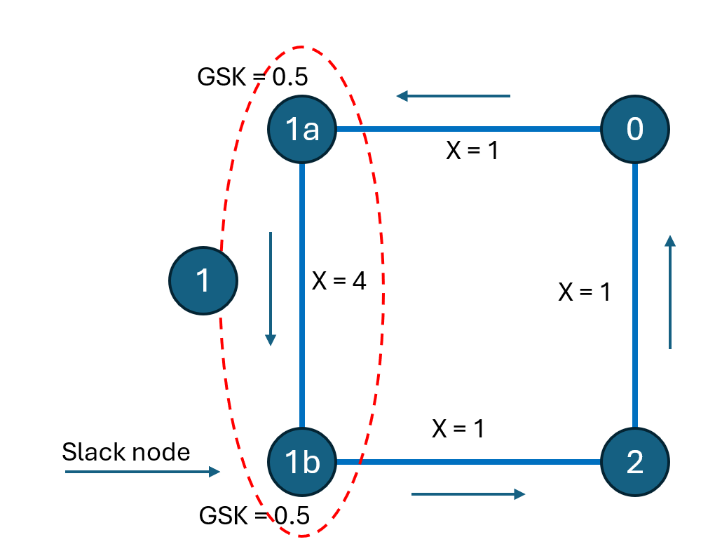
To account for physical network constraints, we revisit the three-zone market but introduce more detail: zone 1 is now represented by two sub-nodes, 1a and 1b, connected by an internal link, which may become congested.

PTDF Matrix and Flow Allocation

In power systems, flows across the network are governed by the Power Transfer Distribution Factor (PTDF) matrix. This matrix relates injections at nodes to flows on links in a linearized model.

• Each row in the PTDF matrix corresponds to a link in the network
• Each column corresponds to a node
• Entry PTDF_ij describes how much flow is induced on link i by injecting 1 MW at node j (with the slack node compensating)

The total flow on any link is then the sum of the effects of injections at all nodes, weighted by their respective PTDF values. This follows directly from the principle of superposition in linear systems.

In our case, we use the following assumptions:

• All external links (between zones) have a reactance of 1 ohm
• The internal link within zone 1 has a reactance of 4 ohm
• Node 1b is selected as the slack node

With these parameters, we can compute the full PTDF matrix for the four-node network. (For a detailed method, refer to the earlier post on PTDF calculation.)

---

Full PTDF Matrix

The full PTDF matrix describes how injections at each node (0, 1a, 1b, 2; 1b selected as slack node) affect flows on each link (including the internal one). Here’s the table governed from the impedances of the full network:

PTDF matrix. Zone/Node: Link:	0	1a	1b	2
0	2/7	-4/7	0	1/7
Internal	2/7	3/7	0	1/7
1	-5/7	-4/7	0	-6/7
2	-5/7	-4/7	0	1/7

Aggregating to Zones Using GSK

To reduce the model back to three zones, we consolidate nodes 1a and 1b into a single zone (zone 1). This requires applying a Generation Shift Key (GSK) to describe how internal nodes contribute to the zone’s net position.

Here, both 1a and 1b are assigned a GSK of 0.5, meaning they each account for half of zone 1’s net injection.

Since node 1b (the slack) contributes zero to all flows, only the 1a values affect the result, and they are halved. The consolidated PTDF matrix (zones 0, 1, 2 vs. links) becomes:

PTDF matrix. Zone: Link:	0	1	2
0	2/7	-2/7	1/7
1	-5/7	-2/7	-6/7
2	-5/7	-2/7	1/7

Internal Constraint in Zone 1

To express the internal constraint on the link between 1a and 1b (within zone 1) in terms of zone net positions, we use the following formula:

Flow on internal link:

(2⁄7) × NP₀ + (3⁄14) × NP₁ + (1⁄7) × NP₂

PTDFs comes from the “Internal” row in the full PTDF matrix. Note the factor 0.5 from the GSK for node 1a, imposed on the second term. To ensure this internal link does not exceed its capacity, we impose the constraint:

(2⁄7) × NP₀ + (3⁄14) × NP₁ + (1⁄7) × NP₂ ≤ RAM

Here:

• NP_i is the net position of zone i
• RAM is the Remaining Available Margin of the internal link, i.e. its maximum allowable flow

Simulating the three-zone model with constrained flows

The three-zone model from the earlier blog post has now been extended as described above, while keeping the original supply and demand curves to allow for a clear, head-to-head comparison. The key difference is that we now maximize welfare subject to an additional constraint: the internal link must not become overloaded.

Let’s explore how this affects the outcome under different scenarios.

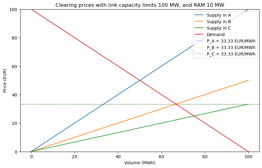
No congestion anywhere

The first scenario considers a case with no congestion. In other words, both the RAM of the internal link and the capacity C of the interconnecting links are sufficiently large to avoid any bottlenecks. This allows the system to operate purely according to economic optimization.

The results in this scenario are identical to those of the previous three-zone model, with one important exception: the flows. Net positions, welfare, production, consumption and prices remain unchanged, but the actual power flows differ because they are now determined by the PTDF matrix.

We observe that the largest flow occurs directly from the low-cost zone 2 to the high-cost zone 0. Due to the higher impedance in zone 1, less power is routed through that path.

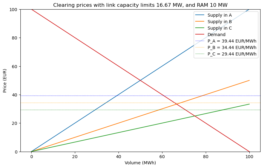
Congestion on interconnect links

If we now reintroduce the capacity limit of 16.67 (as used in the original three-zone model), we observe that it is no longer possible to transfer enough power from zone 2 to zone 0 to fully equalize the prices. The PTDF determined flow is restricted by the capacity constraint C, resulting in a price difference between the zones.

Link 2, which connects nodes 2 and 0, becomes the limiting factor in this case. This illustrates the direct impact of the network’s physical properties, such as line impedances, on how power can flow through the system.

Importantly, the internal congestion within zone 1 is not limiting in this scenario, it remains non-binding despite being part of the model.

Congestion on zone 1 internal link

Now, let’s introduce a congestion on the internal link within zone 1 by setting the RAM to 4 MW, while keeping the interconnecting links unconstrained. As shown in the table, the flow on the internal link is now limited to 4 MW, making it a binding constraint and the new bottleneck in the system.

This leads to an interesting phenomenon: price splitting occurs between the zones even though the interconnecting links are not congested. The internal bottleneck within zone 1 alone is enough to disrupt price convergence across the system.

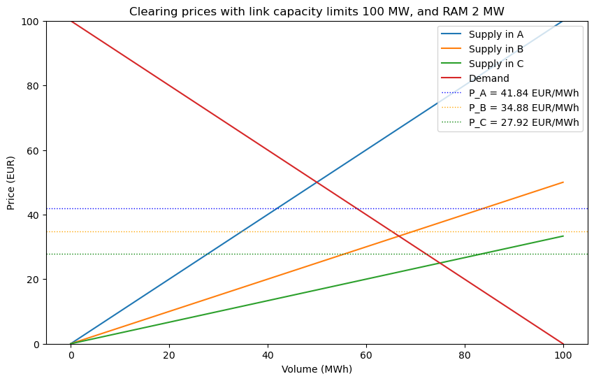
More congestion on internal link

Let’s take it a step further and decrease the RAM to just 2 MW. Now something even more interesting happens: the internal congestion in zone 1 becomes even more dominant, significantly reshaping the flow pattern and price formation across the entire network.

The most notable feature here is that we now see a flow from the more expensive zone 1 to the cheaper zone 2. Since the cheapest zone 2 cannot send enough power through zone 1 to zone 0, due to the internal congestion in zone 1, it becomes more effective overall to export more from zone 1 and reroute the power through zone 2 to the expensive zone 0.

Once again, this is a result of economic optimization (welfare maximization) constrained by physical limitations represented by the PTDF matrix. The non-intuitive flow pattern is also accompanied by a negative congestion rent.

Summary

The economic optimization of the three-zone market model from the previous blog post has here been extended to include physical constraints based on network impedances. This introduces several important features:

• The PTDF matrix, derived from network impedances, effectively “locks in” the previously indeterminate flows, making them physically consistent.
• Most power flows from low-cost zones to high-cost zones via the paths of least impedance.
• An internal congestion within a zone can lead to price differences between zones, even when the inter-zonal links are uncongested.
• When the RAM on an internal link is sufficiently small, non-intuitive flow patterns can emerge as the system reconfigures itself to maximize total welfare within the physical limits.

Additional

The algorithm used here is to maximize the total welfare of the system
Welfare = Consumer Surplus + Producer Surplus + Congestion Rent
subject to the following constraints

• Demand and Supply related through their respective functions
• Sum of net positions equal to zero (network balance)
• Zone 1 internal link flow < RAM
• Interconnect link flows < C

The independent variables becomes the demand and net positions in each zone. Supply is given by the condition that Supply = Demand + Net Position. The constraints are formulated as

cons = [
    {'type': 'eq', 'fun': lambda x: x[0] - dem(x[3], k[0])},                   # demand = dem(n,k)
    {'type': 'eq', 'fun': lambda x: x[1] - dem(x[4], k[1])},                   # x[0:3] = demand in each zone
    {'type': 'eq', 'fun': lambda x: x[2] - dem(x[5], k[2])},                   # x[3:6] = net position for each zone
    {'type': 'eq', 'fun': lambda x: x[3] + x[4] + x[5]},                       # sum n = 0 (network balance)    
    {'type': 'ineq', 'fun': lambda x: RAM - abs(np.dot(ptdf_intern, x[3:6]))}, # Zone 1 internal link constraint, ptdf_intern = [2/7, 3/14, 1/7]
    {'type': 'ineq', 'fun': lambda x: C - max(flows(x[3:6]))},                 # Interconnect link constraints
    {'type': 'ineq', 'fun': lambda x: C + min(flows(x[3:6]))}
]

The solver used is scipy.optimize.minimize. Since this solver only handles the primal problem, it cannot directly produce shadow prices related to the constraints. However, shadow prices can be estimated by changing the binding constraint slightly and monitor the change in total welfare.