
Bengt J. Olsson
Twitter: @bengtxyz
LinkedIn: beos
In a previous post, a two zone power market was modelled. The zones were connected with a single link. The zones had identical demand curves but slightly different supply curves, rendering different prices in the two zones. It could be seen that this difference implied a flow from the low cost zone to the high cost zone, by offsetting the production – consumption balance in both zones.
In this blog post the the power market model is extended to three zones, A, B and C, connected with three links in a triangle. Power thus have alternative ways to flow between the zones. This fact has a profound impact on the model as will be seen.
Like in the previous model, the demand-price curve will be the same in all zones, 100 – v, where v is the demand and 100 – v is the corresponding demand price. The supply-price curves will differ in all three zones and will typically look like v * k[A/B/C], where v is the supplied volume at price v * k, where k typically will be 1 for zone A and less than 1 for zones B and C. That is, A will be the most expensive zone and B/C will be cheaper zones.
Here are the equilibrium prices for the three zones when k = 1, 1/2, 1/3 for A, B, and C respectively, and the zones are not connected (link capacity between zones are 0)
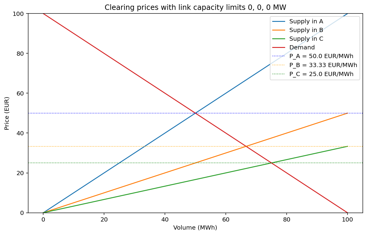
The clearing prices and volumes are different for the three zones as expected. In the expensive zone A, the price is highest, 50 EUR/MWh and hence the cleared volume is the smallest, 50 MWh. Whit cheaper production, the cleared price becomes lower and the cleared volumes larger, just as expected. We can summarize the data for the three zones in this “data structure”
Production k value    : [1, 0.5, 0.33]
Link capacities       : [0 0 0]
Optimal consumption   : [50.   66.67 75.  ] Total: 191.67
Optimal production    : [50.   66.67 75.  ] Total: 191.67
Optimal flow          : [0. 0. 0.]
Prices                : [50.0, 33.33, 25.0]
Net positions         : [0. 0. 0.]
Total welfare         : 9583.33
Let’s introduce two new cases, where the capacity is increased to 5 and 100 MW respectively, for all links. This will result in these two scenarios after total welfare optimization:
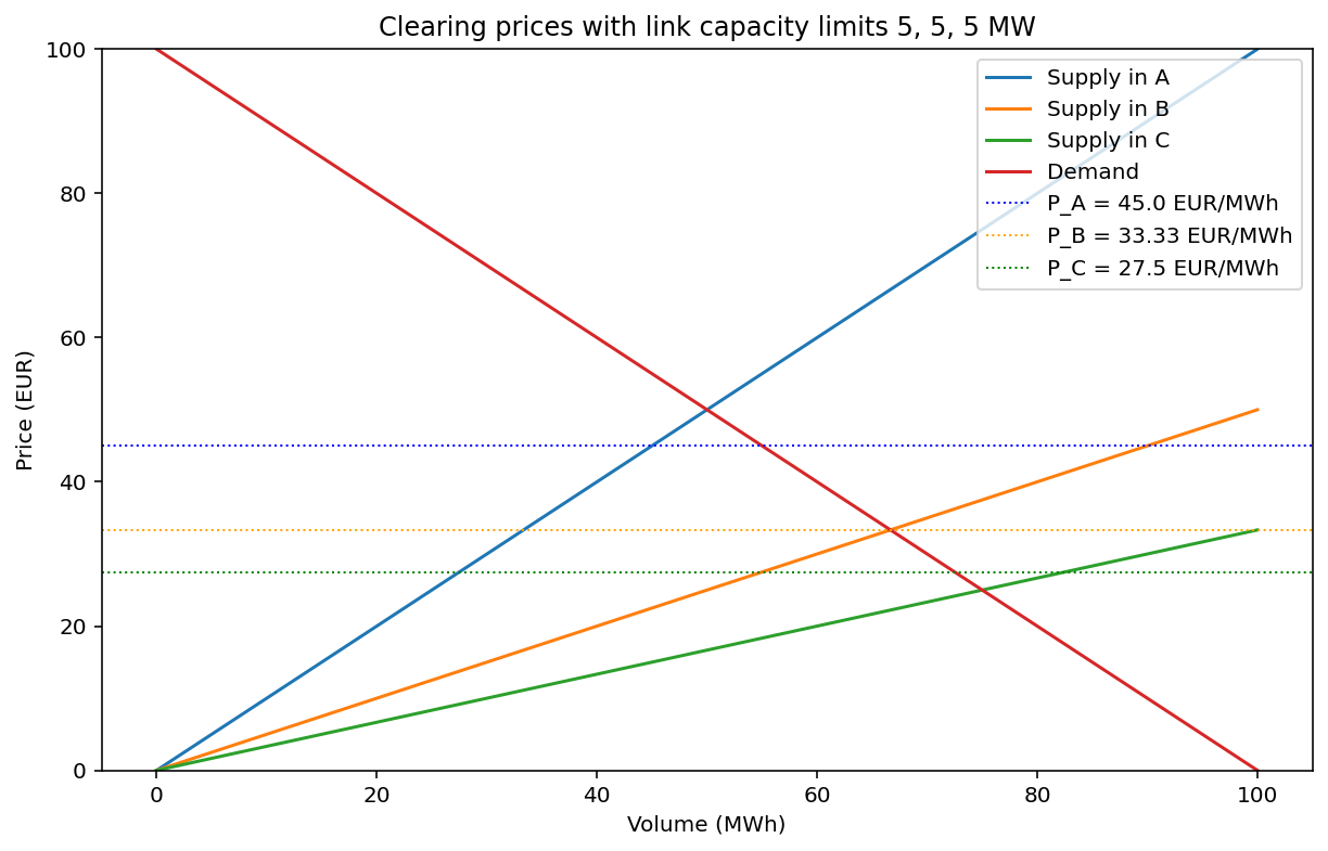
Production k value    : [1, 0.5, 0.33]
Link capacities       : [5 5 5]
Optimal consumption   : [55.   66.67 72.5 ] Total: 194.17
Optimal production    : [45.   66.67 82.5 ] Total: 194.17
Optimal flow          : [-5. -5.  5.]
Prices                : [45.0, 33.33, 27.5]
Net positions         : [-10.   0.  10.]
Total welfare         : 9795.83
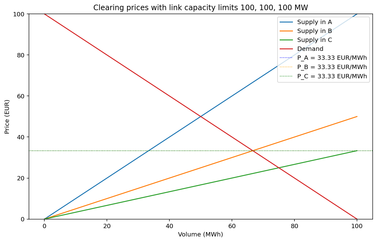
Production k value    : [1, 0.5, 0.33]
Link capacities       : [100 100 100]
Optimal consumption   : [66.67 66.67 66.67] Total: 200.0
Optimal production    : [ 33.33  66.67 100.  ] Total: 200.0
Optimal flow          : [-11.11 -11.11  22.22]
Prices                : [33.33, 33.33, 33.33]
Net positions         : [-33.33   0.    33.33]
Total welfare         : 10000.0
In the first, left, scenario with 5 MW links between the zones we can see that the net positions changes slightly, that is zone A becomes a net importer with 10 MW and zone C becomes a net exporter with 10 MW. For this particular demand/supply situation, B becomes “neutral” with respect to import/export. We can also see that the links are fully utilized, with C supplying 5 MW to both A and B, B receives 5 MW from C and sends 5 MW to A (and thus have net import/export of zero) and finally A receives 5 MW from both B and C. The change in net positions imply a corresponding change is zonal prices. A, with net import becomes cheaper, B is neutral both in net position and price, while C becomes more expensive. The total welfare increases also from the nominal, zero link capacity, case.
When we increase the link capacity to 100 MW, links are no longer constrained. Prices converges to 33.33 EUR/MWh in all zones, and A and C get their optimal net positions of -33.33 and 33.33 MW respectively. We can also see that the total welfare is now maximized to 10 000. The totally consumed and produced energy is 200 MWh out of 300 MWh possible.
Flows versus net positions
One interesting observation is that it is the net positions, not the flows directly that sets the constraints in the model. What is conserved for each zone is the balance between production, consumption and net import/export (net position), in accordance with Kirchhoff’s current law. The net position is given by the flow out of from the zone minus the flow in to the zone: NP = Fout – Fin. This makes the flows to some degree in-determined. If a term “delta” is added to both Fout and Fin this term will cancel out in the calculation of NP. Above the flows (in the non-constrained case) are given as -11.11, -11.11, and 22.22, giving net positions -33.33, 0, and 33.33. But if we lower the link capacities C to for example 16.67 MW instead of 100 we get the following result:
Production k value    : [1, 0.5, 0.33]
Link capacities       : [16.6667 16.6667 16.6667]
Optimal consumption   : [66.67 66.67 66.67] Total: 200.0
Optimal production    : [ 33.33  66.67 100.  ] Total: 200.0
Optimal flow          : [-16.67 -16.67  16.67]
Prices                : [33.33, 33.33, 33.33]
Net positions         : [-33.33   0.    33.33]
Total welfare         : 10000.0
Everything is the same except the flows! Consumption/Production, prices, net positions and welfare is the same. The only difference is the flows. In fact the optimization added a term “delta” as described above with a value of -5.55 to all flows in order to fit all flows under the 16.67 MW capacity limit. Another way to look at it is that in the second case, less power flows directly from the cheap zone C to the expensive zone A, but is instead routed to A via B. Since no physical characteristics is taken into account, these two paths are equivalent in this model. In reality, the impedances of the links and other physical factors will decide the actual paths for the flows (and then we’re in the realm of the “flow-based” constrained model).
If, however, the capacity limit is further lowered, the links start to constrain the needed flows to get the optimal net positions, as can be seen in the 5 MW capacity case above. The links are here fully utilized and there is no way to add or subtract any “delta” without violating the capacity constraints.
As a summary it can be said that the classic zone model with fixed capacity links (also known as the ATC, “Available Transmission Capacity”, model), the outcome of the total welfare optimization are zonal prices and net positions, but not necessarily flows between between zones (unless links are constrained). To fully account also for flows, further physical aspects of the power system must be taken into account.
Since EUPHEMIA only provides net positions and prices for each bidding zone, it is up to the TSO’s to manually make sure that power can flow in accordance with physical constraints and the net positions. One way to provide uniquely determined flows is to introduce Flow Based constraints. But then the welfare optimization becomes much more complex. In this blog post I have built out this 3-zone model with flow-based constraints.
However, I think the above example gives a good intuitive understanding for the difference between net positions and flows in the NTC world.