
Bengt J. Olsson
Twitter: @bengtxyz
LinkedIn: beos
Update 2023-04-16: Added a section about the nuclear fueled “Local power” scenario in the end after the Summary.
The Finnish TSO Fingrid Oy recently published a report describing four possible future scenarios for the Finnish power system 2035 and 2045. The scenarios are
- Power to Products – Value enhanced production of hydrogen based products
- Hydrogen from Wind – Exporter of hydrogen
- Windy Seas – Offshore wind power production
- Local Power – Leaner scenario with local nuclear power production
In this blog post, we will examine the “Power to Products” scenario for 2035, as the report is more detailed for 2035 than for 2045, making it easier to compare apples to apples with our model. This scenario contains a lot of wind power and a lot of hydrogen production, but still quite low flexibility. There are no large hydrogen storage facilities so the otherwise useful hydrogen production flexibility cannot be fully relied upon to offset variations in wind and solar power.
Power to Products scenario
In this scenario, Fingrid outlines a future where Finland produces clean energy with wind power, mainly on land but also offshore. A large part of the energy will be used for new industries, mainly by using hydrogen as a raw material to produce electrofuels/materials/chemicals. No major export of hydrogen is planned, rather an export of refined hydrogen-based products instead.
Unlike other hydrogen producing scenarios, we cannot expect hydrogen production to be a great flexibility resource to use when supply is scarce. Instead, the rest of the power system must be more flexible.
The consumption and production numbers for this scenario from the report are given below.
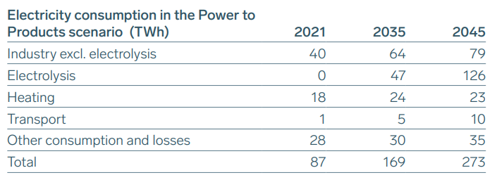
Consumption
169 TWh consumption, out of which 47 is for hydrogen production, leaves 122 TWh for other consumption. In our model we will set a fixed consumption (that varies sinusoidaly over the year) corresponding to 122 TWh before demand flexibility is applied. The demand flexibility is expressed as a percentage that the consumption can be decreased in times with low power production (and hence high power prices). The actual consumption will hence be lower than the 122 TWh nominal consumption due to this flexibility.
It is a bit difficult to assign a number on the flexibility here based on the report data. But based on Figure 16 and Table 15 we will use 20%. This is a rather high number (especially here were there is no time limit for this flexibility, it endures as long as needed).
Hydrogen is produced from electrolyzers. The power “window” that the 7.2 GW elctrolyzers use is adjusted such that 47 GWh is produced, corresponding to approximately 75% capacity utilization. This in accordance to the report. This “window” is partly within the “consumption profile” which is the consumption that the production is balanced with. The other part of the electrolyzer window uses excess energy that would otherwise be exported or curtailed. For our production statistics this window is divided as 5.55 GW withing the consumption profile and 1.65 GW above this profile. Typically hydrogen production within the consumption profile is stable, and above the production is opportunistic.
Hydrogen production flexibility is two-fold: Above the consumption profile hydrogen is only produced when excess power is available. If available power is below the consumption profile we can reduce the hydrogen production up to a certain percentage of the power window within the profile (here 5.55 GW).
Based on Figure 16 we should use 30-40% flexibility but this is a tad much since we require the hydrogen to have a steady production rate. We’ll use 20% here as well.
Hydrogen produced is feed into a 16 GWh hydrogen store. Each hour a certain amount is extracted from the store. Both feed in and feed out have to respect the hydrogen stores max and min limits. This is a relatively small store that demands a steady production to get a steady flow of hydrogen to the industrial consumers.
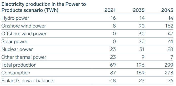
Production
2035 the report envisions 196 TWh to be produced from various power sources. Of these 140 TWh comes from wind and solar power. Now this report is a little bit different in that these 140 TWh are “effective” in the respect that curtailed energy is not included. Usually total production is reported and then how much is curtailed. But from table 14 in the report it is mentioned that 10% of the renewable energy production is curtailed. Thus we conclude here that the total wind + solar production is about 155 TWh and that 15 TWh of these are curtailed to get 140 TWh effective energy. Arbitrarily we divide the 15 TWh curtailed energy to be 2 TWh solar and 13 TWh wind energy and hence our model will assume that the total renewable production is 120 + 13 = 133 TWh wind energy and 20 + 2 = 22 TWh solar energy before curtailment.
“Merit order” of dispatchable sources
In the model wind, solar and nuclear power is considered as must run power sources, and hydro plus thermal power sources are considered dispatchable. Also flexible power sources as battery energy storage, import and export as well as consumption and hydrogen production flexibilities are dispatchable to balance the must run power sources.
Since the model is not including price modelling an “intelligent merit order” of dispatching the flexible power sources is used when balancing the must run sources. Roughly the order looks like this.
Deficiency of must run sources:
Dispatch merit order: Hydro > Thermal > Hydrogen production flex > Load flex partly > Import > Load flex partly > Energy Storage discharge> Deficit
Excess of must run sources:
Dispatch merit order: Energy Storage charging > Hydrogen production from excess power > Export > Curtailment
The flexible sources are dispatched in the above order, subject to their capacity constraints, until balance is reached. If balance is not reached we get a deficit situation or curtailment respectively. The merit order is not perfect and in the real world some intermixing between the flexible sources happens for cost reasons. But intuitively we can understand that this a sensible merit order. For example in deficiency situations, import will probably more expensive than to dispatch own hydro and thermal resources. Likewise you will probably produce hydrogen from excess wind or solar instead of exporting it for a low price.
Must run sources
Wind, solar and nuclear are considered must run sources. Wind and solar power statistics is taken from ENTSO-E for Denmark 2020-2021. Denmark has a mix of onshore and offshore wind energy and also solar statistics from at least similar latitudes as Finland. The Danish onshore and offshore wind power is added hour by hour to provide a common wind statistics. This statistics is then scaled linearly in such way that the sum matches the assumed wind energy production, 133 TWh per year in this case. The same is done with the solar statistics to get 22 TWh per year production.
Nuclear power is modeled with four reactors of approximately 1 GW that individually transitions between working and non-working states according to a Markov chain model. Overlaid is also a 30 days maintenance down period for each reactor one time per two years starting randomly during the summer half of the year. Together this gives 31 TWh (in accordance with the report) and a 87% capacity factor.
Simulation
The parameter values from the report are inserted into the model together with the deducted parameters. The latter are
- The wind/solar energy additions as above
- 20% consumption flexibility
- 20% hydrogen production flexibility
- 4 GW / 10 GWh battery energy storage
Import/Export limits of 6.67 GW are used in accordance with the report. This will have implications on the net export as we will see.
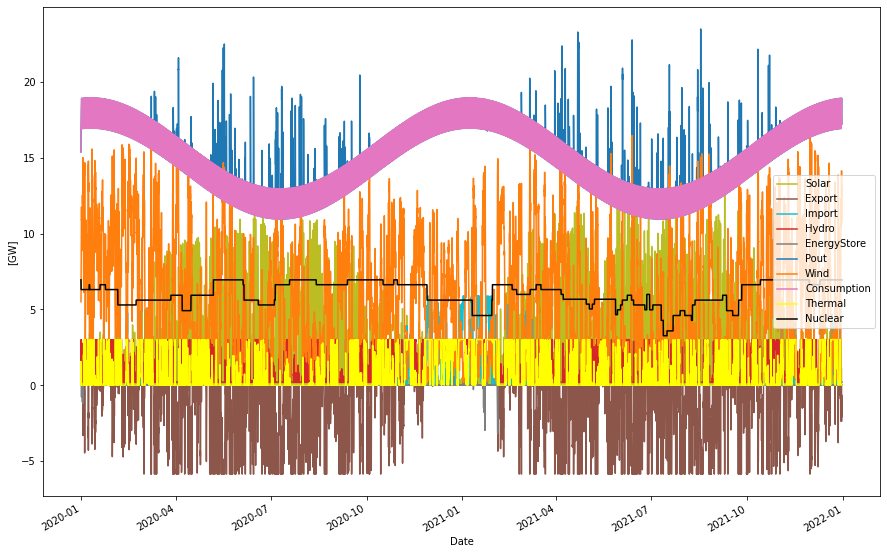
Now let’s rund the simulation (about 20 seconds for two years!) Here is the result
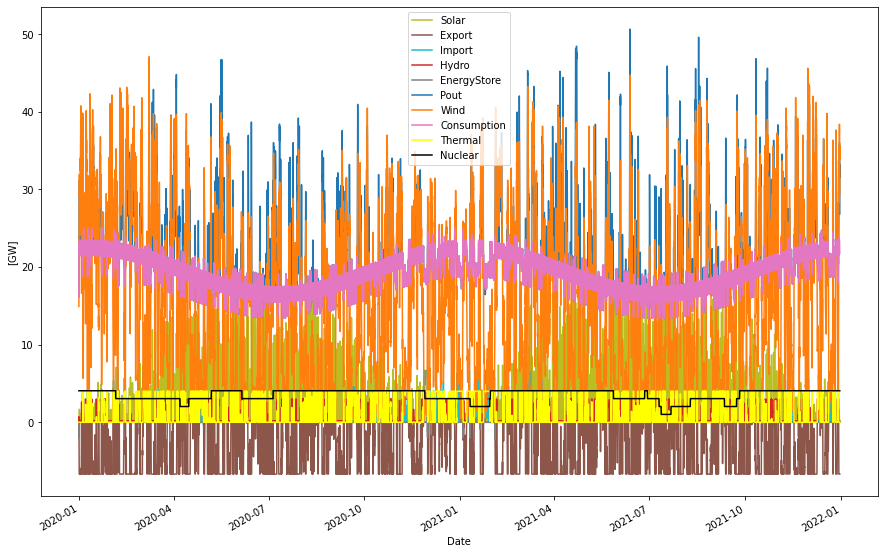
Supplied power per year:      208.84 TWh
Consumption per year:         166.96 TWh
Produced hydro per year:       12.06 TWh
Produced thermal per year:     10.70 TWh
Produced wind per year:       133.09 TWh
Produced solar per year:       22.00 TWh
Produced nuclear per year:     31.00 TWh
Nuclear capacity factor:        86.98 %
H2 production per year:        47.13 TWh
H2 store size                   0.02 TWh
Capacity electrolyzers:         7.20 GW
Cap. util. electrolyzers:      74.72 %
Def. store in/out cap           4.00 GW
Def. store storage cap         10.00 GWh
Curtailed per year             21.56 TWh
Deficit per year                0.01 TWh
Max shortage:                   1.85 GW
Max overshot:                  33.01 GW
Import per year:                4.26 TWh
Export per year:               24.59 TWh
Consumption flexibility:       20.00 %
Hydrogen flexibility:          20.00 %
Nominal non-H2 cons.          122.17 TWh
Real non-H2 cons.             119.83 TWh
Flexibility loss:               1.91 %
Hydro + thermal amounts to about 23 TWh together, which is the same as in the report, however in this simulation a bit more thermal and less hydro is produced. Wind, solar and nuclear is per design the same as in the report (after adding “removed” power as described above for wind and solar). 47 TWh hydrogen is produced and delivered through the 16 GWh store, using 7.2 GW of electrolyzers with 75% utilization factor.
The battery energy store almost handles deficiency situations, there is a tiny bit left in January 2021 where the battery store wasn’t enough to cover for the deficit. But this falls under the error margin.
Now the big difference vs the report. In this simulation more than 15 TWh is curtailed, rather around 21.5 TWh. This extra curtailment eats from the net export balance that now becomes around 20.3 TWh instead of 26 TWh in the report. But this was with 6.67 GW import/export capacity. If we change these numbers to 9 GW as only change and re-run the simulation we get
Curtailed per year             15.56 TWh
Import per year:                4.39 TWh
Export per year:               30.60 TWh
Nothing else is significantly changed. But now we have the correct curtailment (15 TWh) and a net export of 26 TWh just like in the report. Should be interesting to find out what this discrepancy depends on.
Anyway we keep the 6.67 GW import/export limits and look at Januari 2021 in detail to better see the dynamics.
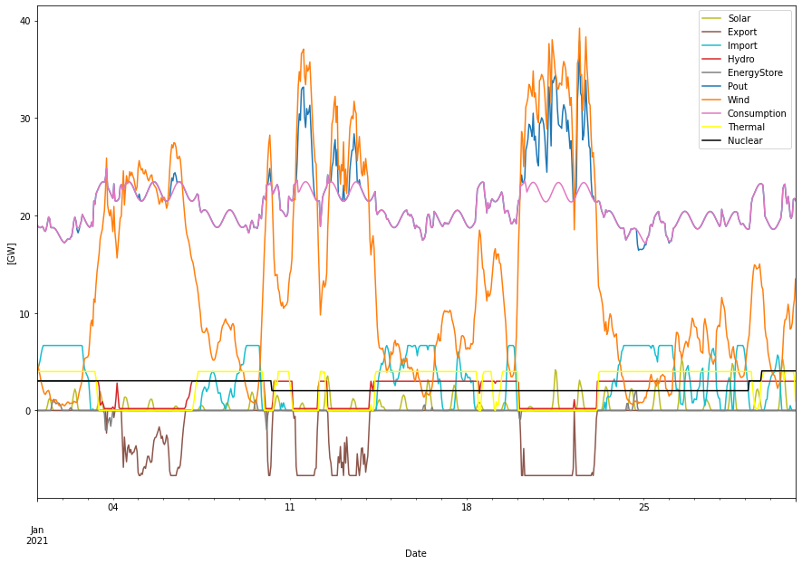
We can see curtailment when the sourced power (blue line) is above the purple demand line and a small deficit at January 24 when the blue line is below the purple line. The small grey peaks the 24th are the battery discharging trying to cover the deficit, but suddenly the energy store is empty and the deficit becomes a fact. (An even smaller deficit can be spotted on January 2). Corresponding energy store (10 GWh) is here
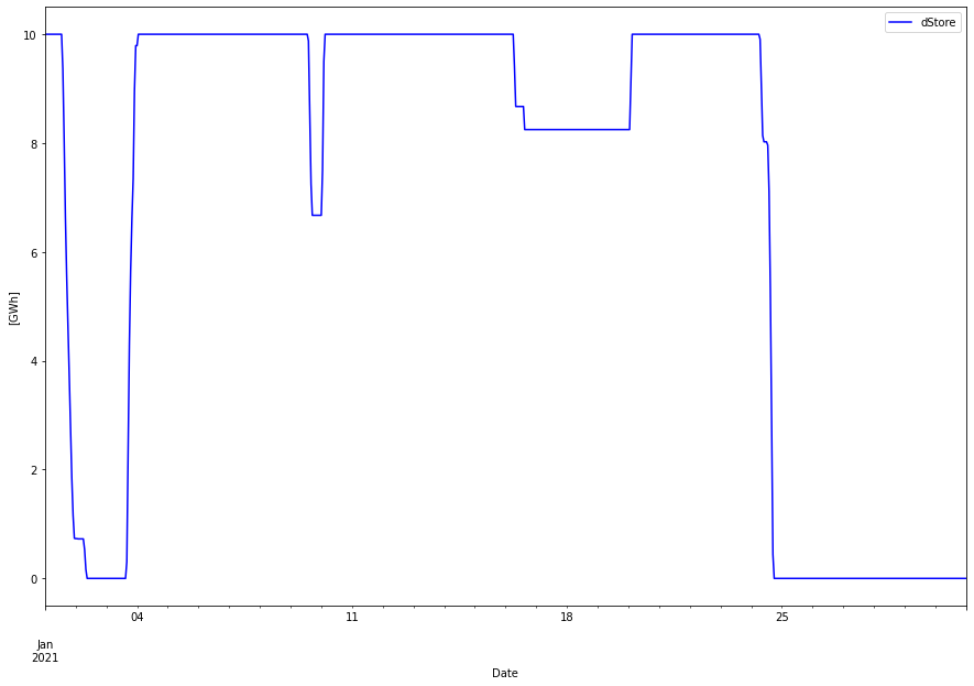
Hydrogen production
Hydrogen production is quite straightforward. With only 20% flexibility in the production there will each hour be at least 5.55 * 0.8 = 4.44 GWh delivered to the store, meaning that this is the minimum amount out of the store. This can be seen in the graph below also for Jan 2021. Red is fill level of store (note that it is after delivery each hour, why it is never seen full, 16 GWh, but rather 16 – 47/8.77 = 10.6 GWh which can be seen as the maximum in the graph). Orange is the delivered amount each hour.
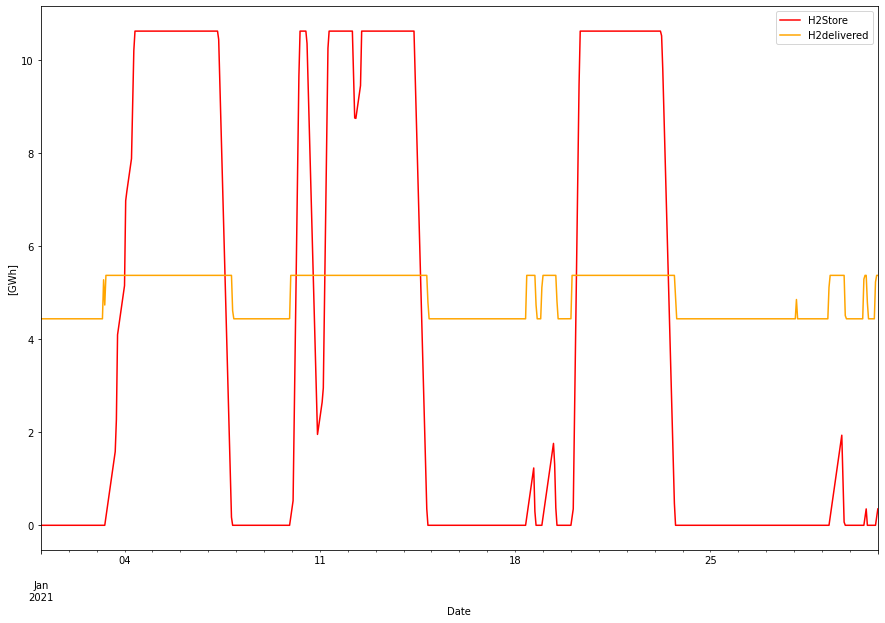
It is clearly seen how the fill level and delivery correlates with the wind peaks above.
Summary
The simple balance model using scaled real wind and solar power data does a good job with recreating the results from the Fingrid’s “Power to Products” scenario for 2035. The only real discrepancy is about the ratio between curtailment and net export, but this could be brought into full alignment by just increasing the import/export limits from 6.67 (from report) to 9 GW. After that the results are almost in perfect agreement.
The scenario seems quite viable in most respects. However 20% flex on the consumption sounds rather much too me at least. Decreasing this to more manageable 10% would incur more periods with real deficits (or black-outs somewhere). But on the other hand if import/export limits are also changed to 9 GW instead of 6.67 GW, 10% flexibility can be handled without deficits.
Even though the net export is high, so is the dependency on import for balancing the must run sources. Whether it is 6.67 or 9 GW there may be competition from other countries for that import energy.
Hydrogen production is straightforward in this case, where it is mostly part of the consumption “baseload” and have a relatively low flexibility. The delivery is stable with a variation of maximum 1 GWh/h and the 16 GWh storage is sufficient (at least from a modelling perspective…).
Update: “Local Power” scenario
2023-04-16
Instead of making an own long blog post on the “Local power” scenario I will just give the results here. Scenario is for 2045 instead of 2035 since we’re dealing with new SMR technology. Given its larger content of stable nuclear base load production (and hence need for less variable renewable production) it produces power to cover the demands without thrills. Here is the breakdown.
Supplied power per year:      138.83 TWh
Consumption per year:         131.29 TWh
Produced hydro per year:       14.40 TWh
Produced thermal per year:      7.47 TWh
Produced wind per year:        49.00 TWh
Produced solar per year:       14.98 TWh
Produced nuclear per year:     52.99 TWh
Nuclear capacity factor:        87.01 %
H2 production per year:        16.00 TWh
H2 store size                   0.02 TWh
Capacity electrolyzers:         1.82 GW
Cap. util. electrolyzers:     100.13 %
Def. store in/out cap           8.00 GW
Def. store storage cap         20.00 GWh
Curtailed per year              1.34 TWh
Deficit per year                0.01 TWh
Max shortage:                   1.36 GW
Max overshot:                  10.00 GW
Import per year:                3.49 TWh
Export per year:                9.70 TWh
Consumption flexibility:        0.00 %
Hydrogen flexibility:           0.00 %
Nominal non-H2 cons.          115.16 TWh
Real non-H2 cons.             115.30 TWh
Flexibility loss:              -0.12 %
The same nuclear power production (31 TWh) as in the “Power to Products” scenario above is assumed, but have also added nine SMRs of 320 MW that with an 87% capacity factor adds additional 22 TWh energy to get a total of 53 TWh nuclear production.
The results agree well with those of the report. Net export is here 6 vs 7 TWh in the report. Both hydro and thermal production is close to the report values.
16 TWh of hydrogen are produced and delivered within the consumption profile with no hydrogen production flexibility (gives 100% capacity utilization of the electrolyzers).
Notable is that I have required no demand flexibility in this simulation (as well as no hydrogen production flexibility). There are hints of deficits during the colder months where the battery storage is not sufficiently large to cover the deficiencies. It is assumed to be 20 GWh which is twice of the amount in the Product to Power scenario since we are here looking at 2045 instead of 2035. But with just some percent of flexibility these deficits disappear altogether.
The Local Power scenario is thus “safer” from a energy security point of view than the Power to Products scenario, with less import dependency and less chance for power deficits. SMR’s are certainly an interesting prospect!