
Bengt J. Olsson
Twitter: @bengtxyz
Norway is blessed with fantastic natural resources. Not only in the fossil space but also in order to produce abundant amounts of clean power. The basis for this is their huge hydro power capacity. We will here use a simple balance model to depict what the Norweigan power system could look like in 2050.
Input data
The input numbers are taken from “Langsiktig markedsanalyse Norden og Europa 2020–2050” and its update. In short it proposes the following consumption/production development:
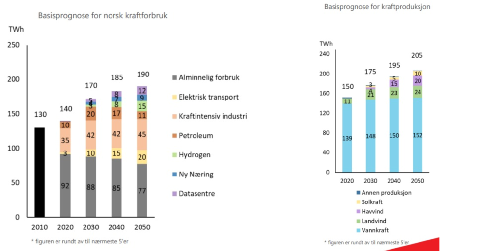
As we can see we expect an increase in consumption from about 140 TWh in 2020, to 190 in 2050. Of the 50 TWh increase, we have almost +20 TWh in the transport sector, +10 TWh in the power intensive industry, about +20 TWh in datacenters and new ventures. On top of this +15 TWh of hydrogen production is anticipated. This adds up to +65 TWh but there is also a decrease of about -15 TWh in general consumption, providing the net +50 TWh increase.
On the production side, we can see an increase of all renewable power sources, hydro, on- and off-shore wind and solar power. For hydro the increase is due both to expected climate effects (more rain…) and increased efficiency in many smaller hydro power stations. New off-shore wind (20 TWh) and an increase of on-shore wind power up to 24 TWh is expected. 10 TWh of solar is also anticipated.
Model
We now need to “mold” the data into the model in order to do the simulation. This is the way it is done.
Scale wind and solar power to the target levels
In order to provide a statistics of wind and solar power to the model, Danish ENTSO-E data is used. The reasons for this are several. First, the amount of Norweigan data on off-shore wind power and solar power are miniscule, why scaling such data would most probably amplify statistical irrelevant variations. Denmark on the other hand has “stable” data for both on/off-shore wind power and solar power for the years 2020 and 2021 that we are using here. While the wind and solar patterns likely are different between Denmark and Norway, they should probably be like enough to provide a meaningful simulation. After all, the simulation is just a sample in an ensemble of different weather outcomes, and in another sample we really could have this statistics in Norway as well. I.e close enough to provide useful results.
Model hydro power
The hydro power is simply modelled as a “perfect” source that can ouput between 5 – 25 GW as needed for balancing the other sources with the consumption. The span is obtained just by visually inspecting what the actual output has been during the last years. (If someone can propose better limits I would be happy to know).
No attempt has been made to model the fill level in the reservoirs, it is expected that the reservoir can supply the the total energy need, here 152 TWh. (The model can actually coarsely simulate the hydro storage levels as described in this (swedish) twitter thread, but need further input work for that, maybe to be added later).
Consumption
Consumption is modeled with a sinus curve with maximum in winter and minimum in summer. Amplitude of this sine is ±4 GW and the offset 21.7 GW corresponds to 190 TWh consumption. This variation over the year captures pretty well the behavior over the year today and it is assumed that we will have the same seasonal consumption pattern 2050. If needed, a daily consumption variation, modelled as a sinus curve with max at 15:00 and min at 03:00 and with an amplitude of ±2.5 GW can be added to capture the day/night variation to some extent. This variation does not really affect the power balance, except from that it could cause stronger overshots (in the night) or deficits (during day). But from a power/energy balance it is not really necessary to use this day/night variation.
Import/Export
Import and export is notoriously difficult to model in this balance model, since import and export are “power sources” that are dispatched after hydro power to balance whatever is still un-balanced. That is, if hydro power capacity (25 GW here) is exhausted, import is needed to balance the rest. Conversly, if we have an excess from “must run” sources (wind/solar) plus minimum water dispatch (here 5 GW) we export the rest. Of course limits can be set on import and export capacities, if these are exceeded we instead have, deficit and curtailment respectively.
This strict “merit order” of dispatching power sources in this balance model i.e.
- Must run sources (here wind and solar power)
- Hydro power
- Import/Export
- (Deficit/Curtailment)
kind of reflects the merit order in terms of increasing “cost” for the type of dispatched power (i.e. cost wind/solar < hydro < import/export < deficit/curtailment) and hence eliminate the need to do a very complex price computation for dispatching the right kind of power. Such a computation would be completely out of scope for this kind of modelling. But this fixed merit order does quite a good job of dispatching the right kind of power in the right order, and this is because in general the cost really follows the ladder above.
This was a long explanation to reach to the fact that import and export is difficult to handle in this model, since it will exhaust the possibilities to dispatch hydro power before importing/exporting. In this model it means that whatever the consumption is, the model will try to dispatch as much hydro power as possible to balance the power each hour. But in the real world, there will be an exchange between dispatching hydro or use imported power, and likewise, instead of saving water it may be dispatched for export purposes. This model, with its rigid merit order dispatch, can not model these effects.
What we can do instead to capture for example the export is to explicitly add the exported amount as consumption instead. Then the model will dispatch hydro power to cover for this export. For example it seems like Statnett allocates about 15 TWh (205-190) for export. If we assume that this difference is export we can just add it to the consumption, that then changes from 21.7 to 23.4 GW instead. And that is what we do in the model.
Hydrogen production
Hydrogen production, which here amounts to 15 TWh, must also be treated specially. This since hydrogen production is really a natural source for flexibility. If a power deficit occurs (or electricity becomes really expensive which is actually the same thing) it is possible to decrease the amount of hydrogen produced and use hydrogen from a buffer store instead. There are some aspects of this that need some extra consideration.
First question is how flexible you can make hydrogen delivery before it hurts the users? Large industrial hydrogen users may have processes that needs to run continuously and cannot shut down without large impact on its business. Hence output from the buffer stores need to be within limits. This implies a) limits on the hydrogen production variation and b) that the size of the buffer store is big enough, or rather a combination of both.
The other question is how to use the electrolyzer capacity for making hydrogen? There are two possibilities here
- The electrolyzers are within the “consumption profile”, that is considered like any other end consumer of electricity. This means that the electrolyzer expect to work with a 100% capacity factor.
- The electrolyzer uses excess power. We then have to define “excess” power. In this model excess power would be power that otherwise would be curtailed. In terms of this model we then “dispatch” the electrolyzer according to this merit order
Must run > Hydro > Export > Electrolyzer > Curtailment
(In the other way when there is a deficit situation the merit order looks like this instead
Must run > Hydro > Electrolyzer flex > Import > Deficit )1
In the Norwegian case things are again simplified. Having all this hydro power makes it easy to balance both consumption and the variable wind/solar power. In fact there is really no excess energy since the hydro power alone can balance between production and consumption. So in this case the electrolyzers will work according to option 1 above, that is within the consumption profile and with 100% capacity factor (at least almost as we will see). This in its turn makes large hydrogen buffer stores unnecessary (again we will see that a smaller store could be beneficial to have anyway).
Note that the model looks at the national level and there are no provisions to handle internal transmission bottlenecks inside Norway.
Simulation
Power dispatch
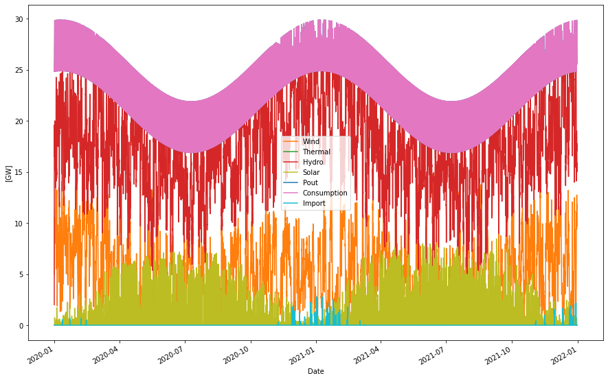
Running a simulation of the model power system for 2050-2051 it would look as follows
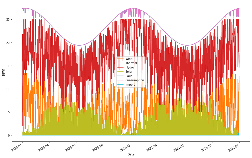
Supplied power per year:      205.16 TWh
Consumption per year:         205.12 TWh
Produced hydro per year:      151.25 TWh
Produced wind per year:        44.20 TWh
Produced solar per year:        9.69 TWh
Produced nuc/bio per year:      0.00 TWh
H2 production per year:        15.03 TWh
- From excess power:            0.00 TWh
- Within consump. profile:     15.03 TWh
H2 out per year:               15.03 TWh
Cap. util. electrolyzers:      98.04 %
Curtailed per year              0.00 TWh
Deficit per year               -0.00 TWh
Max shortage:                  -0.00 GW
Max overshot:                   0.00 GW
Import per year:                0.01 TWh
Export per year:                0.04 TWh
The system is nicely in balance. No power overshots or deficits. It produces power in line with was is proposed in the figure from Statnett above. Note that the consumption here includes 15 TWh that are exported as explained above. The import is very low which partly is because the electrolyzers are flexing down its production of hydrogen when power supply is low. This can be seen by the downward peaks in the pink consumption graph. In real life there could possibly be an exchange such that electrolyzer flex is smaller and we import to cover the deficit instead. It is really a cost issue, but it is also a very small effect here, we could probably live with either case.
In this picture we amplify what happens between December 15 – January 15 when the system is under high load
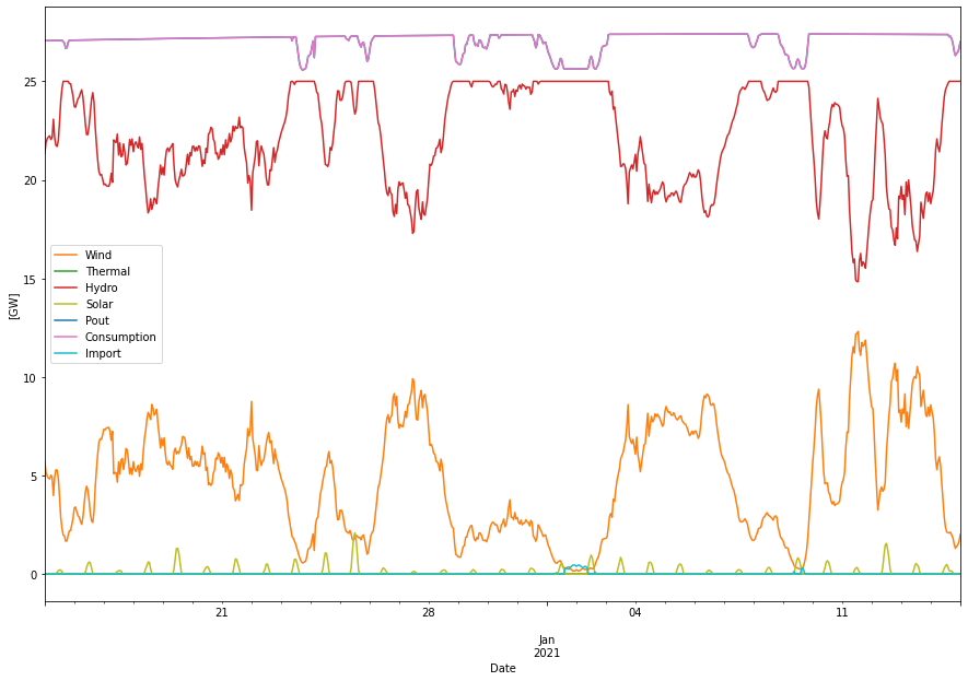
We can see how hydro power is balancing the wind power and how hydrogen flex also helps with the balancing. On January 1-2 we can see that hydrogen flex is exhausted and hence a small amount of import is needed. We can also see in-significant amounts of solar power as well (maybe more a sign of the Danish heritage of the solar statistics…).
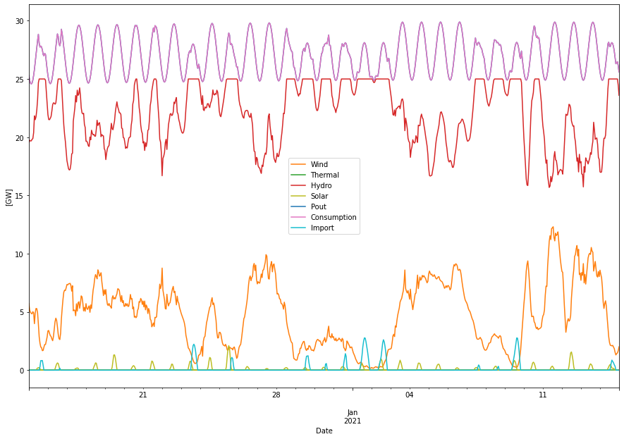
If we add day/night consumption variation we see that more import is needed during daytime (even though the accumulated level is still small).
Hydrogen production
Now let’s have a look at the hydrogen production. As we mentioned above in the model section the electrolyzer capacity is fully within the consumption profile of the model and hence works at full capacity all the time. Except the few times were it flexes down production to save power (only at winter time in this simulation). When flex is included we get a healthy capacity factor of 98% for the electrolyzers. With this high capacity factor the needed electrolyzer capacity to generate 15 TWh yearly is only 1.75 GW.
If we look at the hydrogen delivery we can inspect the storage level of a hydrogen store of 400 GWh that starts (and ends) with a fill level of about 150 GWh.
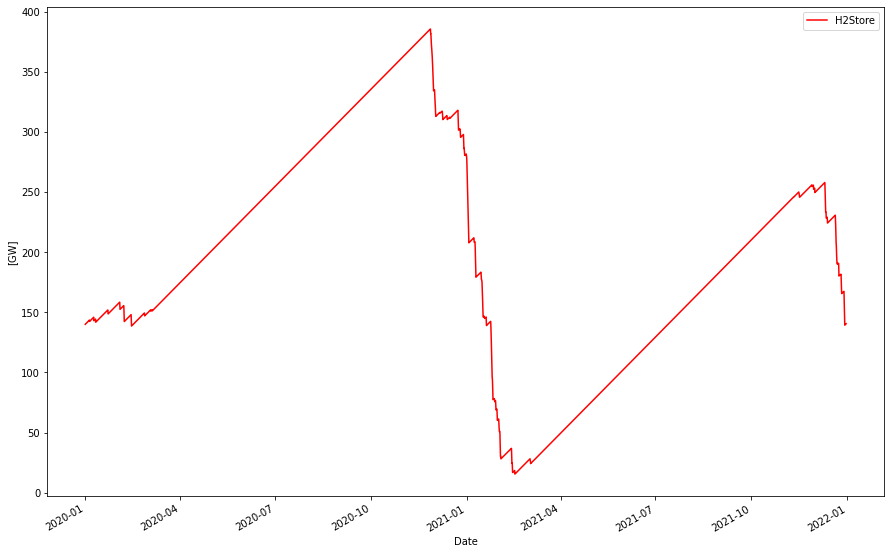
It is filled by the electrolyzer hydrogen production and emptied at a constant rate equal to the mean production rate (about 1.7 GW). We can see that a stock is build up to handle that the production is muted when it flexes down to save power during the low wind circumstances during December/January in this simulation.
It is noteworthy that even though we have an almost perfect hydrogen production flow, we still need a relatively large hydrogen store of 400 GWh. That makes you think about how much would be needed in terms of storage if the production is following the variability of weather dependent power, or if only excess power peaks would be used for hydrogen production?
If we include day/night consumption variation that we saw “drained” the hydrogen production even more during winter time, the store size increases to +500 GWh.
Conclusion
We can again see that Norway is blessed with the right natural resources for expanding their power system with more renewable power sources, i.e. more hydro, wind and solar. The anticipated energy mix is 74% hydro, 21% hydro and 5% solar. Norway will be able to expand to a 190 TWh consumption level, export 15 TWh yearly, produce 15 TWh of green hydrogen using 1.75 GW electrolyzer capacity working at almost 100%.
All this while still having a plannable dispatch of power without significant over-shots or deficits.
The hydrogen production is more or less continuous but may flex down a little during low wind winter days. But also this small production flex leads to the need of relatively large hydrogen stores in order of several hundred GWh on the national level.
Footnotes
- In principle, the export that we here treat as consumption, should be treated in the same way as the hydrogen production, that is as a flexible consumer that will throttle down when power is scarce. Since we need a fix “merit order” in this model we have to decide which resource to flex down first. In most cases this would probably be the export, since you want to disturbe the hydrogen production flow as little as possible. Hence the resulting “deficit” merit order would be
Must run > Hydro > Export flex > Electrolyzer flex > Import > Deficit
In this simulation this would have resulted in that we would have had the same consumption dips as now, but these would be dips in the export, and the hydrogen production would have been untouched with 100% capacity factor.